
Rで2変量(2次元)データを LOESS(locally estimated scatterplot smoothing) により、但し関数 loess {stats} を使用せずに平滑化します。
参照しました資料(以降、参照資料)は以下の通りです。
- https://www.itl.nist.gov/div898/handbook/pmd/section1/dep/dep144.htm
- https://www.itl.nist.gov/div898/handbook/pmd/section1/pmd144.htm#tcwf
- https://simplyor.netlify.app/loess-from-scratch-in-python-animation.en-us/
始めに参照資料1にありますサンプルデータ(同資料中の x と y )を関数 loess {stats} を使用せずに平滑化し、同じく参照資料1で示されています LOESS回帰 の結果(同資料中の Regression Function Value )と比較します。
Figure 1 の黒点が参照資料1の x と y の点、そして赤点は span = 7/21(0.33)、degree = 1( the local model is a straight line ) とし、ウエイト関数を tricube weight function とされている LOESS回帰 の結果(同資料中の Regression Function Value )の点です。
なお、tricube weight function は以下の通りです。
\[\begin{eqnarray} w(u) = \begin{cases} \left(1 - |u|^3\right)^3 & |u| < 1 \\ 0 & |u| \geq 1 \end{cases}\end{eqnarray}\]
x [1] 0.5578196 2.0217271 2.5773252 3.4140288 4.3014084 4.7448394
[7] 5.1073781 6.5411662 6.7216176 7.2600583 8.1335874 9.1224379
[13] 11.9296663 12.3797674 13.2728619 14.2767453 15.3731026 15.6476637
[19] 18.5605355 18.5866354 18.7572812y [1] 18.63654 103.49646 150.35391 190.51031 208.70115 213.71135 228.49353
[8] 233.55387 234.55054 223.89225 227.68339 223.91982 168.01999 164.95750
[15] 152.61107 160.78742 168.55567 152.42658 221.70702 222.69040 243.18828RegressionFunctionValue [1] 20.59302 107.16030 139.76740 174.26300 207.23340 216.66160 220.54450
[8] 229.86070 229.83470 229.43010 226.60450 220.39040 172.34800 163.84170
[15] 161.84900 160.33510 160.19200 161.05560 227.34000 227.89850 231.55860library(ggplot2)
g <-
ggplot(mapping = aes(x = x)) +
geom_point(mapping = aes(y = y)) +
geom_line(mapping = aes(y = RegressionFunctionValue), colour = "red", linewidth = 0.1) +
geom_point(mapping = aes(y = RegressionFunctionValue), colour = "red", size = 2) +
theme_minimal()
g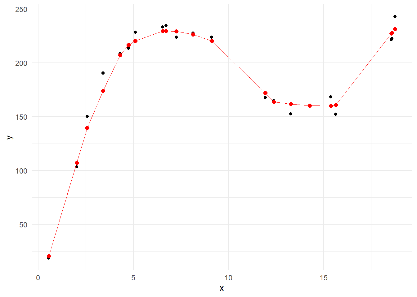
それでは、Rで参照資料1中の Regression Function Value ( Figure 1 の赤点)を再現します。
なお、LOESS回帰 による偏回帰係数 \(\hat{\boldsymbol{\beta}}\) の算出は以下の通りです。 \[\begin{eqnarray} \mathbf{WX}\hat{\boldsymbol{\beta}} & = & \mathbf{Wy} \\ \mathbf{X'WX}\hat{\boldsymbol{\beta}} & = &\mathbf{X'Wy} \\ \mathbf{X'WX}\hat{\boldsymbol{\beta}} & = &\mathbf{X'Wy} \\ \left(\mathbf{X'WX}\right)^{-1}\mathbf{X'WX}\hat{\boldsymbol{\beta}} & = & \left(\mathbf{X'WX}\right)^{-1}\mathbf{X'Wy}\\ \mathbf{I}\hat{\boldsymbol{\beta}} & = & \left(\mathbf{X'WX}\right)^{-1}\mathbf{X'Wy}\\ \hat{\boldsymbol{\beta}} & = & \left(\mathbf{X'WX}\right)^{-1}\mathbf{X'Wy}\\ \end{eqnarray}\]
library(dplyr)
n <- length(x)
span <- 7 / n
W <- b <- list()
bandwidth <- floor(n * span)
X <- as.matrix(cbind(1, x))
y_hat <- vector()
for (iii in seq(n)) {
  distance.all <- abs(X[, 2] - X[iii, 2])
  ind <- order(distance.all, decreasing = F)
  distance <- distance.all[ind] %>% head(bandwidth)
  distance.max <- max(distance)
  u <- (distance / distance.max)
  W[[iii]] <- (1 - u^3)^3 %>% diag()
  local.X <- X[ind %>% head(bandwidth), ]
  local.y <- y[ind %>% head(bandwidth)]
  b[[iii]] <- solve(t(local.X) %*% W[[iii]] %*% local.X) %*% t(local.X) %*% W[[iii]] %*% local.y
  y_hat[iii] <- local.X %*% b[[iii]] %>% .[1, ]
}
cbind(RegressionFunctionValue, y_hat)
RegressionFunctionValue y_hat
[1,] 20.59302 20.59302
[2,] 107.16030 107.16031
[3,] 139.76740 139.76738
[4,] 174.26300 174.26304
[5,] 207.23340 207.23338
[6,] 216.66160 216.66159
[7,] 220.54450 220.54448
[8,] 229.86070 229.86069
[9,] 229.83470 229.83471
[10,] 229.43010 229.43012
[11,] 226.60450 226.60446
[12,] 220.39040 220.39041
[13,] 172.34800 172.34800
[14,] 163.84170 163.84166
[15,] 161.84900 161.84897
[16,] 160.33510 160.33508
[17,] 160.19200 160.19199
[18,] 161.05560 161.05559
[19,] 227.34000 227.33996
[20,] 227.89850 227.89853
[21,] 231.55860 231.55856y_hat が関数 loess {stats} を使用せずに求めた LOESS回帰 による平滑化の結果です。
Regression Function Value と y_hat は一致しています。
Figure 1 に y_hat を重ねます。
g + geom_point(mapping = aes(y = y_hat), size = 4, col = "green", alpha = 0.4)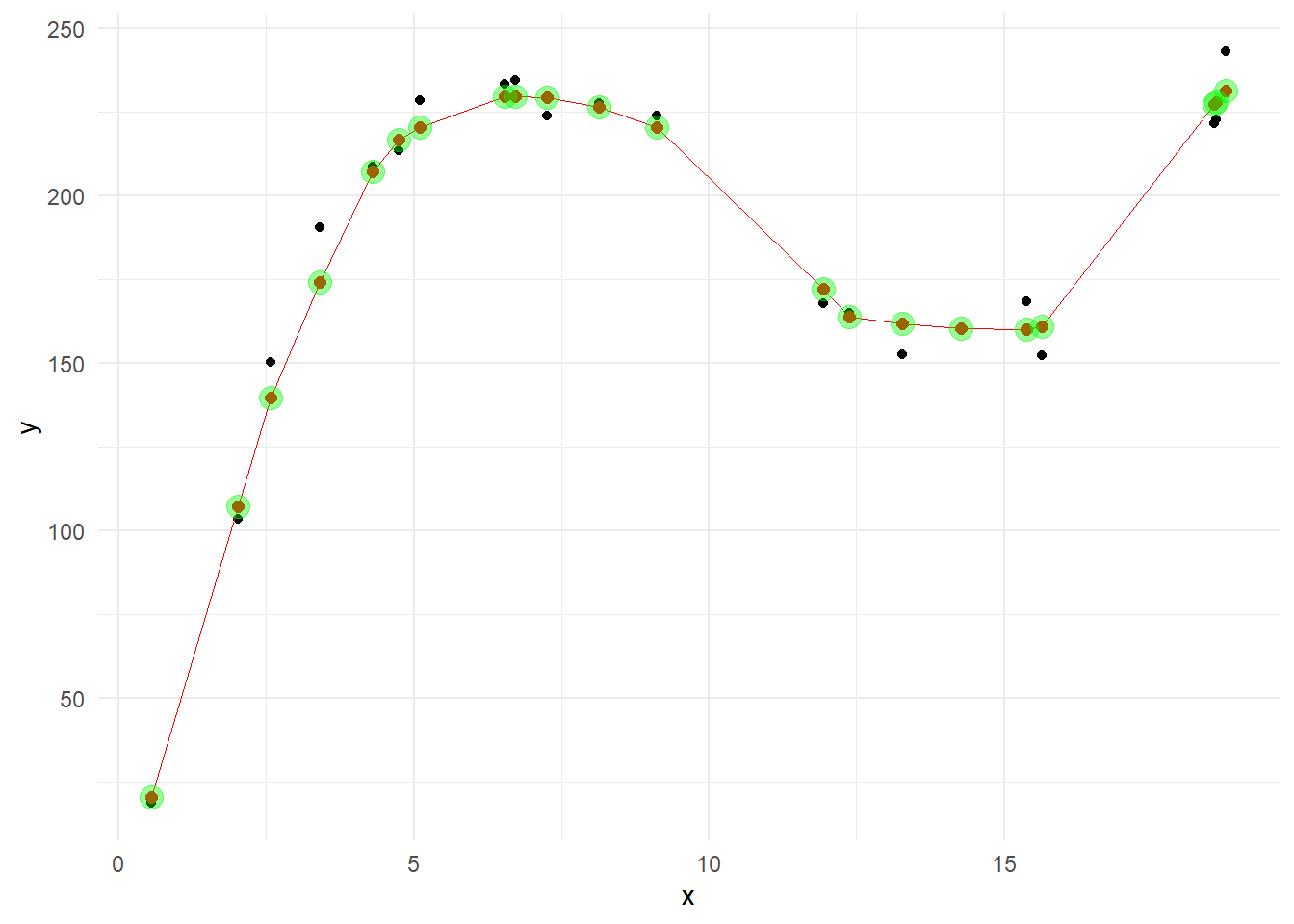
一致していることが確認できます。
続いてもう一つサンプルデータを作成します。
Figure 3 の黒点が作成しましたサンプルデータです。
set.seed(20240709)
n <- 300
x1 <- runif(n = n) %>%
  sort(decreasing = F) %>%
  round(4)
x2 <- x1^2
b1 <- 5
b2 <- -4
b0 <- 4
y <- b0 + b1 * x1 + b2 * x2 + rnorm(n = n, sd = 0.1)
span <- 0.3
g <- ggplot(mapping = aes(x = x1, y = y)) +
  geom_point(size = 1) +
  theme_minimal()
g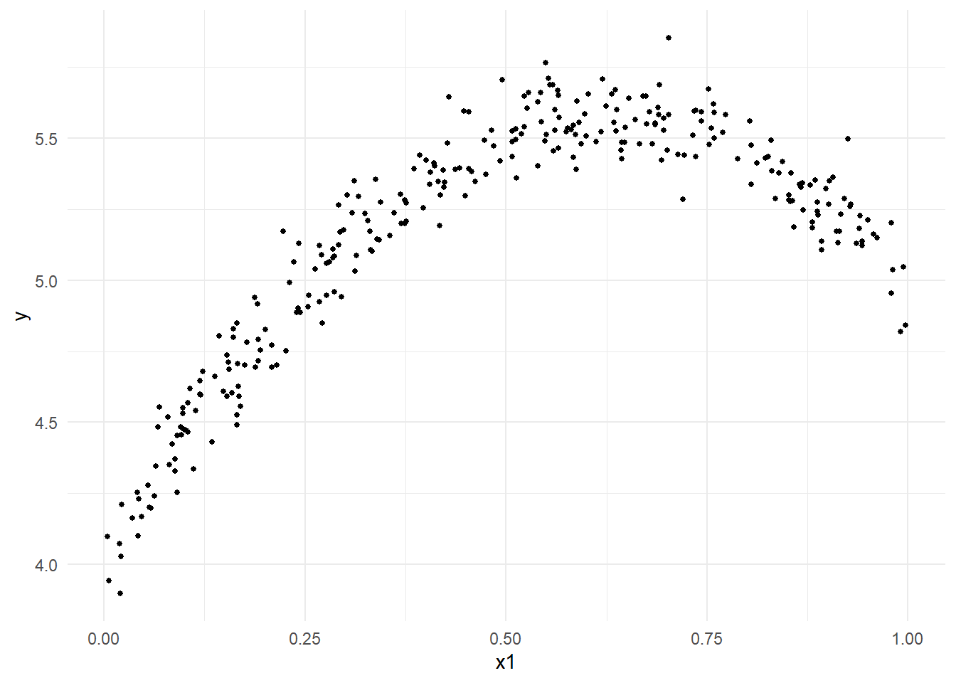
ここでも関数 loess {stats} を利用せずに LOESS回帰曲線 を求めます。
今回は 次数2の多項式 で平滑化します。
Figure 4 の赤点が平滑化した点です。
W <- b <- list()
bandwidth <- floor(n * span)
X <- as.matrix(cbind(1, x1, x2))
y_hat <- vector()
for (iii in seq(n)) {
  distance.all <- abs(X[, 2] - X[iii, 2])
  ind <- order(distance.all, decreasing = F)
  distance <- distance.all[ind] %>% head(bandwidth)
  distance.max <- max(distance)
  u <- (distance / distance.max)
  W[[iii]] <- (1 - u^3)^3 %>% diag()
  local.X <- X[ind %>% head(bandwidth), ]
  local.y <- y[ind %>% head(bandwidth)]
  b[[iii]] <- solve(t(local.X) %*% W[[iii]] %*% local.X) %*% t(local.X) %*% W[[iii]] %*% local.y
  y_hat[iii] <- local.X %*% b[[iii]] %>% .[1, ]
}
g + geom_point(mapping = aes(y = y_hat), col = "red", size = 2.0)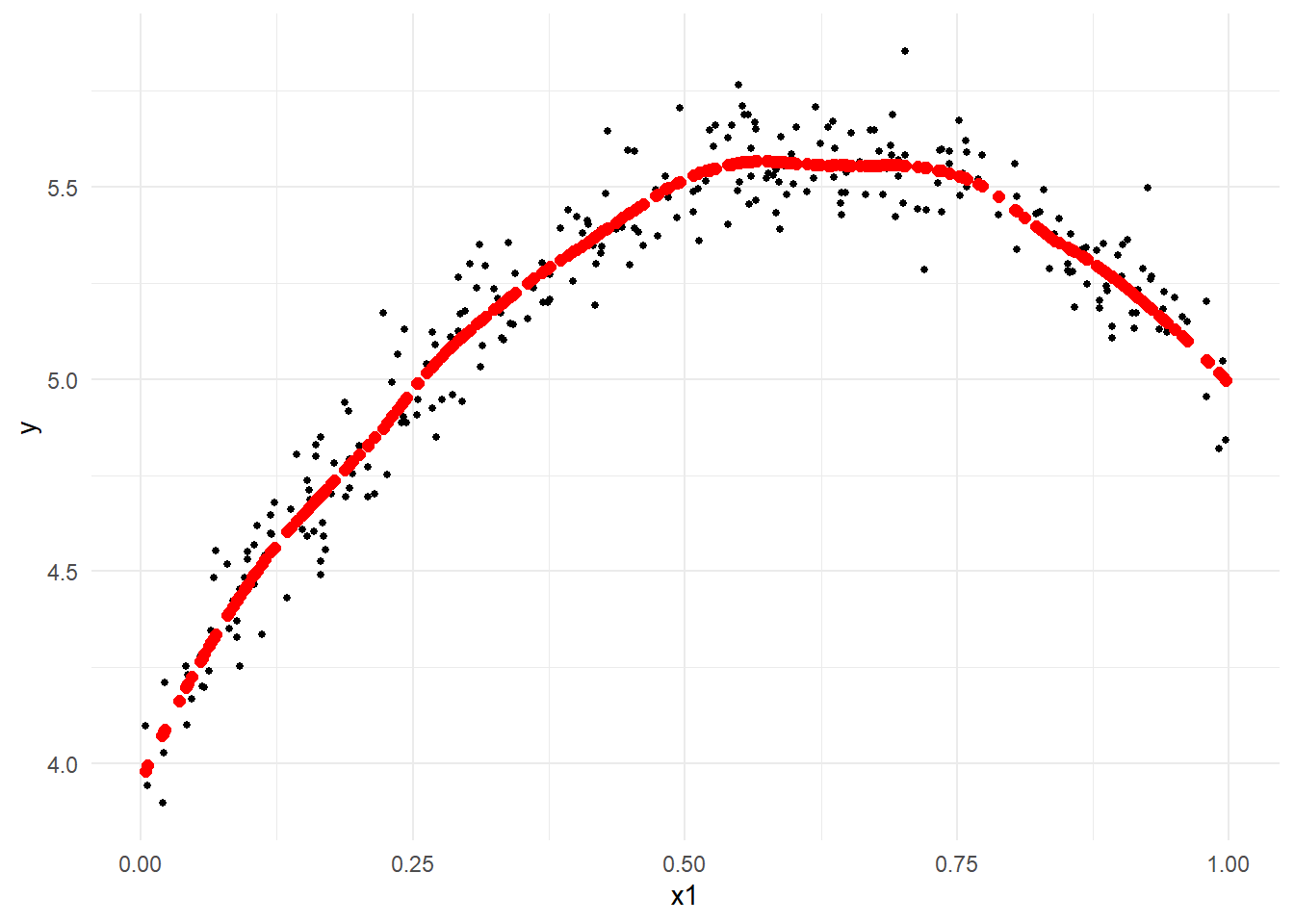
確認のため、geom_smooth を利用した(関数 loess {stats} を利用した)、LOESS回帰曲線 をFigure 4 に重ねます。その際、視認性を向上させるために黒点(サンプルデータ)を除き、赤点の透過度を変更します。
ggplot(mapping = aes(x = x1, y = y)) +
  geom_point(alpha = 0) +
  geom_point(mapping = aes(y = y_hat), col = "red", alpha = 0.3, size = 2.0) +
  theme_minimal() +
  geom_smooth(method = loess, method.args = list(degree = 2, span = span, family = "gaussian", method = "loess"), se = F, linewidth = 1.2)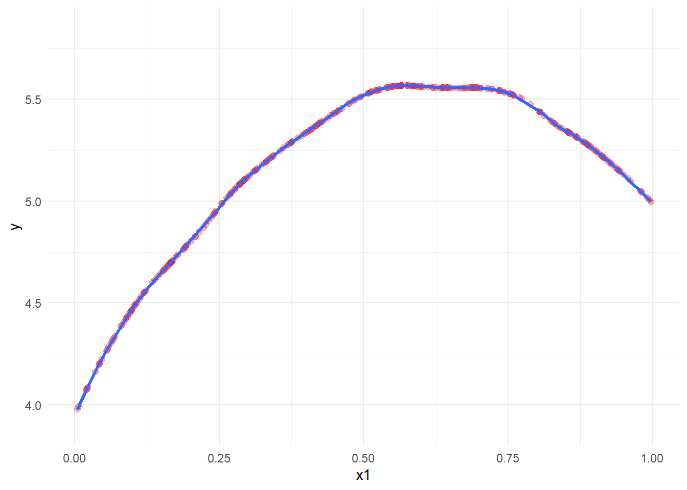
関数 loess {stats} を使用せずに求めた平滑化の結果( y_hat )は geom_smooth で表示した LOESS回帰曲線(青色曲線)に載っている事が確認できます。
以上です。