
ジボット=アンドリュース検定(Zivot Andrews test) により 構造変化を考慮した 単位根検定を行います。
以降の数式、導出は https://www.fbc.keio.ac.jp/~tyabu/keiryo/perron.pdf を引用参照しています。
それでは R で 構造変化を考慮した単位根検定 を行います。
なお、以降有意水準は 5% とします。また、ラグは共通して lag = 3 としていますが本件の場合は数値自体に意味はありません。
始めにサンプルデータ y を作成します。
ベースとするサンプルは 100個(n) の ホワイトノイズ。t が 50(bp) 以降、切片(intercept) を -2、傾き(slope) を 0.25 とした 構造変化 を加えます。
seed <- 20240821
set.seed(seed)
library(dplyr)
library(ggplot2)
n <- 100
t <- seq(n)
bp <- 50
intercept <- -2
slope <- 0.25
y <- rnorm(n) + (intercept + (t - bp) * slope) * (seq(n) > bp)
ggplot(mapping = aes(x = t, y = y, colour = seq(n) > bp)) +
  geom_line() +
  geom_point() +
  geom_smooth(method = "lm") +
  theme(legend.position = "none")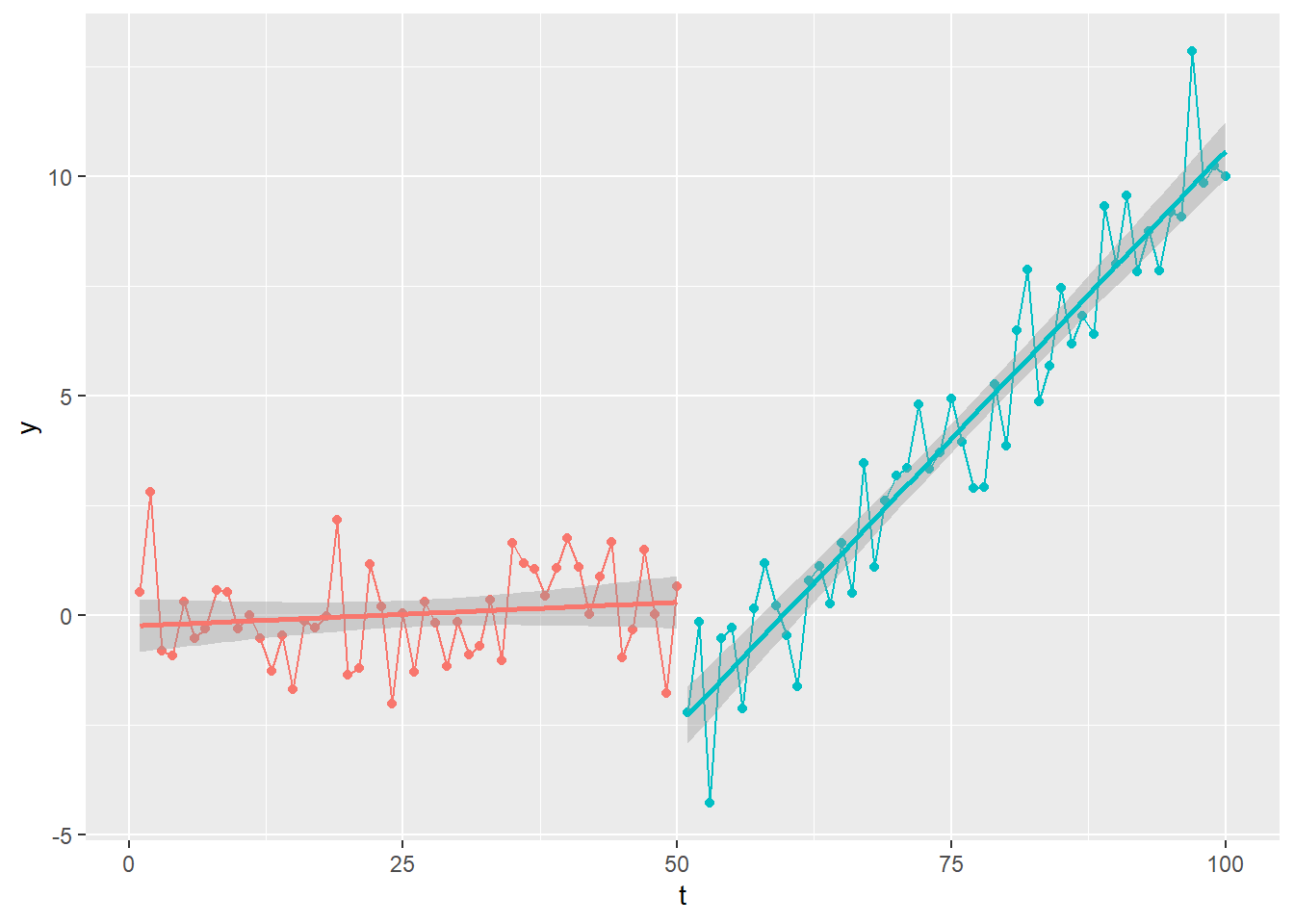
構造変化を考慮しないADF検定 を掛けますと、ベースは ホワイトノイズ ですが 単位根 は棄却されません。
lag <- 3
urca::ur.df(y = y, type = "trend", lags = lag) %>% urca::summary()
###############################################
# Augmented Dickey-Fuller Test Unit Root Test #
###############################################

Test regression trend


Call:
lm(formula = z.diff ~ z.lag.1 + 1 + tt + z.diff.lag)

Residuals:
    Min      1Q  Median      3Q     Max
-3.8809 -0.7900  0.1036  0.7850  3.6112

Coefficients:
             Estimate Std. Error t value Pr(>|t|)
(Intercept) -0.443714   0.336357  -1.319 0.190458
z.lag.1     -0.060284   0.067779  -0.889 0.376146
tt           0.016224   0.007929   2.046 0.043664 *
z.diff.lag1 -0.788531   0.116211  -6.785 1.19e-09 ***
z.diff.lag2 -0.507054   0.125915  -4.027 0.000118 ***
z.diff.lag3 -0.201115   0.105328  -1.909 0.059394 .
---
Signif. codes:  0 '***' 0.001 '**' 0.01 '*' 0.05 '.' 0.1 ' ' 1

Residual standard error: 1.25 on 90 degrees of freedom
Multiple R-squared:  0.4367,    Adjusted R-squared:  0.4054
F-statistic: 13.95 on 5 and 90 DF,  p-value: 4.338e-10


Value of test-statistic is: -0.8894 3.1978 2.8176

Critical values for test statistics:
      1pct  5pct 10pct
tau3 -4.04 -3.45 -3.15
phi2  6.50  4.88  4.16
phi3 8.73 6.49 5.47そこで、構造変化を考慮した単位根検定 として ジボット=アンドリュース検定(Zivot Andrews test) を利用します。
ジボット=アンドリュース検定(Zivot Andrews test) の流れは次の通りです。
- 標本期間の初めから及び最後から15%のデータを構造変化点候補から除きます。
- 構造変化点候補全てについて ペロン検定 により t検定統計量 \(\tau\left(T_B\right)\) を求めます。
- 求めた t検定統計量 \(\tau\left(T_B\right)\) のうち、最小の検定統計量 \(\textrm{inf-}t\) を臨界値と比較します。
それでは始めに構造変化点候補の下限 \(T_{min}\) と上限 \(T_{max}\) を求めます。
T_min <- n * 0.15
T_max <- n * (1 - 0.15)
list(T_min = T_min, T_max = T_max)
$T_min
[1] 15
$T_max
[1] 85よって、構造変化点候補は \(T_B=(15,16,17,\cdots,83,84,85)\) となります。
続いて ペロン検定 により構造変化点候補毎の検定統計量を求めます。
次の ドリフト項、トレンド項 いずれも あり のモデルを考えます。
\[y_t=a_0+\gamma t+\theta_0DU_t+\theta_1DT_t+a_1y_{t-1}+u_t\] 同モデルに対して \[\textrm{H}_0:a_1=1,\,\textrm{H}_1:a_1<1\] とする検定が ペロン検定 です。
構造変化点を bp = 50 とした例を以下に示します。
fun_Perron_test <- function(y, bp) {
  sample.df <- y %>% data.frame()
  sample.df[, 2] <- head(y, -1) %>% c(NA, .)
  sample.df[, 3] <- seq(y)
  y.diff <- y %>%
    diff(lag = 1, differences = 1) %>%
    head(n - 2)
  sample.df <- cbind(sample.df, embed(x = y.diff, dimension = lag) %>% rbind(matrix(nrow = lag + 1, ncol = lag), .))
  sample.df$DU <- c(rep(0, bp), rep(1, n - bp))
  sample.df$DT <- c(rep(0, bp), seq(n - bp))
  sample.df <- sample.df %>% na.omit()
  colnames(sample.df) <- c("y_t", "y_{t-1}", "t", seq(lag) %>% paste0("Δy_{t-", ., "}"), "DU", "DT")
  result.lm <- lm(sample.df) %>% summary()
  return(result.lm)
}
result.lm <- fun_Perron_test(y = y, bp = 50)
result.lm
Call:
lm(formula = sample.df)

Residuals:
    Min      1Q  Median      3Q     Max
-2.5289 -0.7785 -0.0313  0.6663  3.0432

Coefficients:
            Estimate Std. Error t value Pr(>|t|)
(Intercept) -0.54972    0.38817  -1.416 0.160247
`y_{t-1}`   -0.02723    0.19167  -0.142 0.887340
t            0.01999    0.01284   1.556 0.123206
`Δy_{t-1}` -0.08640    0.16781  -0.515 0.607934
`Δy_{t-2}` -0.11131    0.13342  -0.834 0.406394
`Δy_{t-3}` -0.05308    0.09651  -0.550 0.583734
DU          -3.02674    0.75136  -4.028 0.000119 ***
DT           0.25078    0.04669   5.371 6.32e-07 ***
---
Signif. codes:  0 '***' 0.001 '**' 0.01 '*' 0.05 '.' 0.1 ' ' 1

Residual standard error: 1.097 on 88 degrees of freedom
Multiple R-squared:  0.9146,    Adjusted R-squared:  0.9078
F-statistic: 134.6 on 7 and 88 DF,  p-value: < 2.2e-16
\(\textrm{H}_0:a_1=1\) であるため、t検定統計量 は \[(推定値-1)/標準偏差\]として求めます。
(coef(result.lm)[2, 1] - 1) / coef(result.lm)[2, 2][1] -5.359321それでは構造変化点候補毎に ペロン検定 を掛けて、\(\textrm{inf-}t\) を求めます。
fun_Zivot_Andrews_test <- function(y, bp) {
  if (T_min <= bp & bp <= T_max) {
    result.lm <- fun_Perron_test(y = y, bp = bp)
    ((coef(result.lm)[2, 1] - 1) / coef(result.lm)[2, 2]) %>% return()
  } else {
    return(NA)
  }
}
t <- sapply(X = seq(n), FUN = function(bp) fun_Zivot_Andrews_test(y = y, bp = bp))
min_T <- which.min(t)
inf_t <- t[min_T]
list(min_T = min_T, inf_t = inf_t)
$min_T
[1] 50
$inf_t
[1] -5.359321\(\textrm{inf-}t\) は-5.3593207、構造変化点(bp) は50 となりました。
トレンド項あり、ドリフト項あり の場合の \(\textrm{inf-}t\) の 臨界値(Critical Value) を次の資料から引用します。
- Zivot, E., & Andrews, D. W. K. (1992). Further Evidence on the Great Crash, the Oil-Price Shock, and the Unit-Root Hypothesis. Journal of Business & Economic Statistics, 10(3), 251.
| 有意水準 | 臨界値 |
|---|---|
| 1.0% | -5.57 |
| 2.5% | -5.30 |
| 5.0% | -5.08 |
| 10.0% | -4.82 |
| 50.0% | -3.98 |
| 90.0% | -3.25 |
| 95.0% | -3.06 |
| 97.5% | -2.91 |
| 99.0% | -2.72 |
Model (A) permits an exogenous change in the level of the series, Model (B) allows an exogenous change in the rate of growth, and Model (C) admits both changes.
出典: Zivot, E., & Andrews, D. W. K. (1992). Further Evidence on the Great Crash, the Oil-Price Shock, and the Unit-Root Hypothesis. Journal of Business & Economic Statistics, 10(3), 251.
有意水準5% の場合の 臨界値 は -5.08 、\(\textrm{inf-}t\) は -5.359321 ですので、\(\textrm{H}_0:a_1=1\) は棄却されます。
なお、ur.za {urca} を利用して Zivot and Andrews Unit Root Test が行えます。上記 Rコードは 同関数を参考にしました。
urca::ur.za(y = y, model = "both", lag = lag) %>% urca::summary()
################################
# Zivot-Andrews Unit Root Test #
################################


Call:
lm(formula = testmat)

Residuals:
    Min      1Q  Median      3Q     Max
-2.5289 -0.7785 -0.0313  0.6663  3.0432

Coefficients:
            Estimate Std. Error t value Pr(>|t|)
(Intercept) -0.54972    0.38817  -1.416 0.160247
y.l1        -0.02723    0.19167  -0.142 0.887340
trend        0.01999    0.01284   1.556 0.123206
y.dl1       -0.08640    0.16781  -0.515 0.607934
y.dl2       -0.11131    0.13342  -0.834 0.406394
y.dl3       -0.05308    0.09651  -0.550 0.583734
du          -3.02674    0.75136  -4.028 0.000119 ***
dt           0.25078    0.04669   5.371 6.32e-07 ***
---
Signif. codes:  0 '***' 0.001 '**' 0.01 '*' 0.05 '.' 0.1 ' ' 1

Residual standard error: 1.097 on 88 degrees of freedom
  (4 observations deleted due to missingness)
Multiple R-squared:  0.9146,    Adjusted R-squared:  0.9078
F-statistic: 134.6 on 7 and 88 DF,  p-value: < 2.2e-16


Teststatistic: -5.3593
Critical values: 0.01= -5.57 0.05= -5.08 0.1= -4.82

Potential break point at position: 50
検定統計量(-5.3593 )、構造変化点(50) ともに一致しています。
以上です。