Rでロバスト線形回帰影響関数(huber,hampel,bisquare)の比較

ロバスト線形回帰を扱うRの関数 rlm {MASS} について、引数 method を M推定 とした場合における、引数 psi(影響関数) の3つの選択肢、huber、hampel および bisquare それぞれの結果をシミュレーションで比較します。

本ポストは以下の資料を参照引用しています。

前述の psi はロバスト線形回帰における 影響関数 を指定する引数です。

library(ggplot2)
library(dplyr)
library(MASS)
u <- seq(-10, 10, by = 0.01)
bisquare <- psi.bisquare(u)
huber <- psi.huber(u)
hampel <- psi.hampel(u)
data.frame(u, bisquare, huber, hampel) %>%
  tidyr::gather("psi", , colnames(.)[-1]) %>%
  ggplot(mapping = aes(x = u, y = value, color = psi)) +
  geom_line(linewidth = 1) +
  theme_minimal() +
  theme(axis.title = element_blank(), legend.position = "top") +
  scale_color_manual(values = c("red", "green", "black"))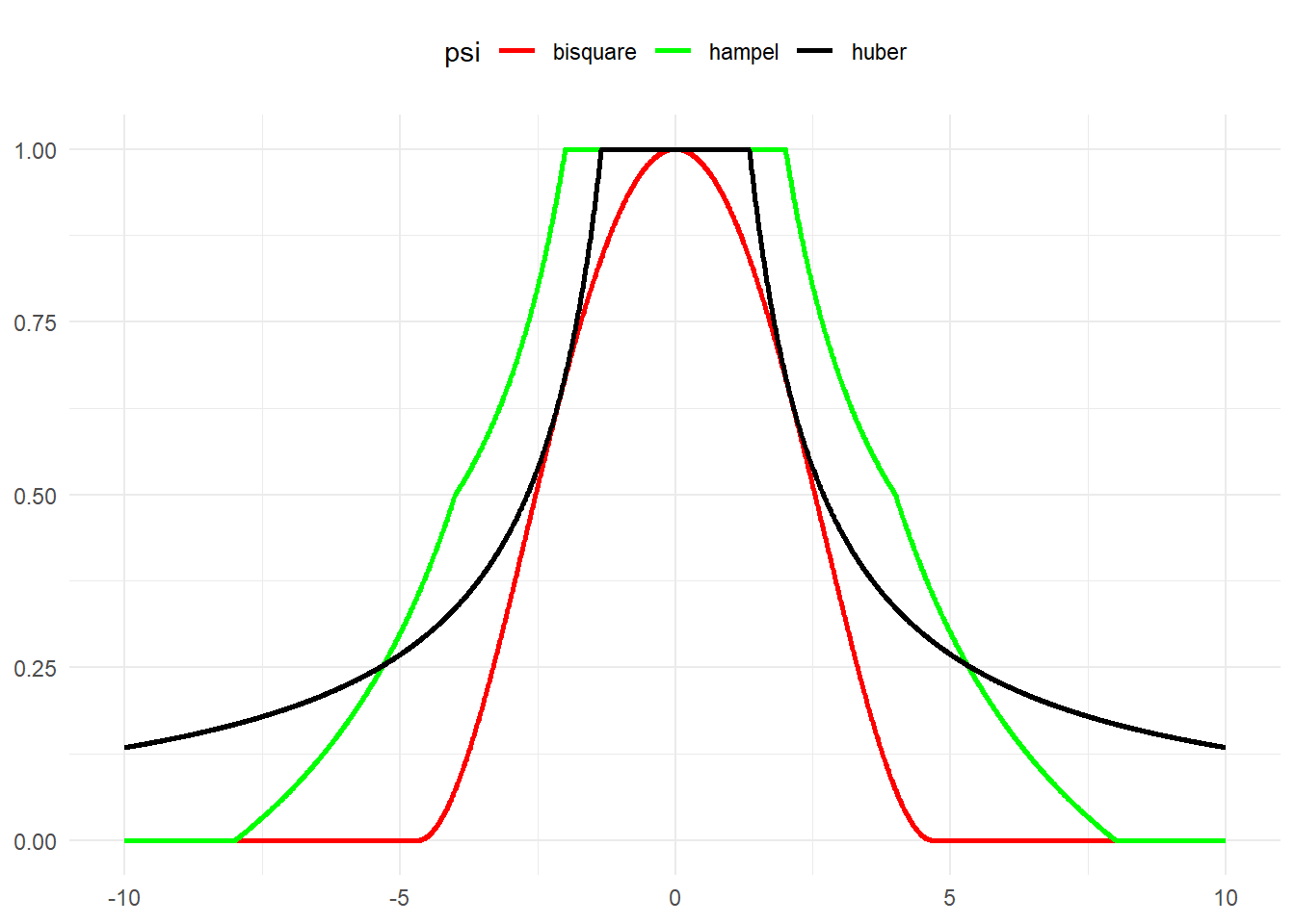

始めに外れ値のあるサンプルデータを生成する関数を作成します。

なお、外れ値は全て「意図的に大きな外れ」とし、かつ回帰直線を「下方向に引っ張る」値とします。

fun_sampledata <- function(seed, n, nout) {
  set.seed(seed)

  # 真のモデル: y = 2 + 3x + ε
  x <- rnorm(n)
  y_true <- 2 + 3 * x
  y <- y_true + rnorm(n, sd = 0.5)

  # 外れ値追加
  id_out <- sample(x = seq(n), size = nout, replace = F)
  y[id_out] <- y_true[id_out] + runif(n = nout, min = -30, max = -20)

  data <- data.frame(x = x, y = y)
  return(data)
}

サンプルサイズは100点。うち5点(全体の5%)を外れ値としたサンプルです。

seed <- 20250328
n <- 100
nout <- 5 # 外れ値数
data <- fun_sampledata(seed = seed, n = n, nout = nout)
glimpse(data)

Rows: 100
Columns: 2
$ x <dbl> 0.02159254, 0.96746160, 1.62807097, 0.97288576, -0.13582887, 1.16101…
$ y <dbl> 2.1168963, 5.0291520, 6.5931878, 4.6417599, 1.9604232, 4.4299156, -3…

外れ度合い をチャートで確認します。

(g0 <- ggplot(data = data, mapping = aes(x = x, y = y)) +
  geom_point())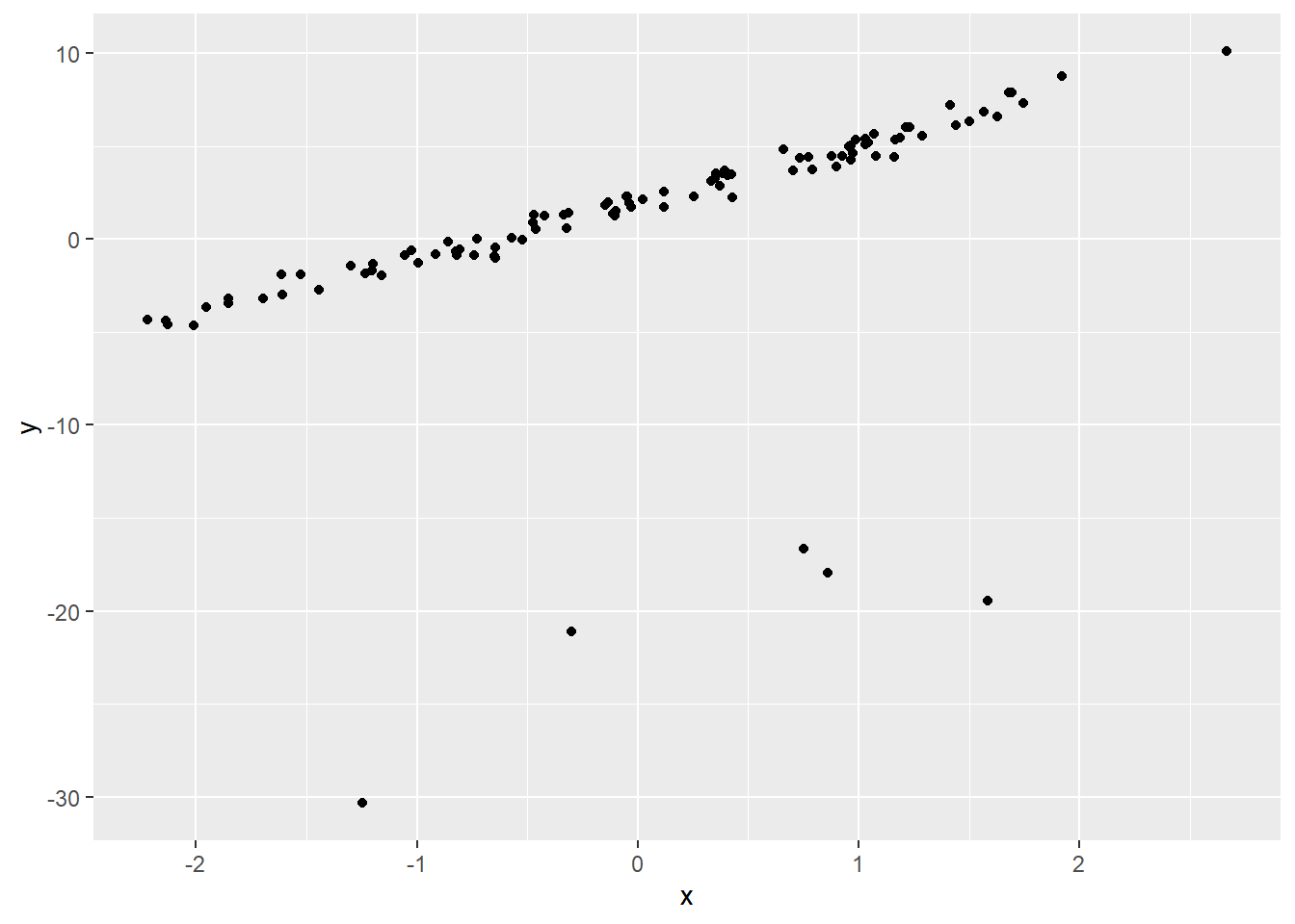

作成したサンプルデータについて、それぞれの影響関数を選択した場合の結果をチャートで比較します。

library(patchwork)
g_bisquare <- g0 + geom_smooth(method = "rlm", se = F, color = "red", method.args = list(method = "M", psi = psi.bisquare, scale.est = "MAD")) + labs(title = "bisquare")
g_hampel <- g0 + geom_smooth(method = "rlm", se = F, color = "red", method.args = list(method = "M", psi = psi.hampel, scale.est = "MAD")) + labs(title = "hampel")
g_huber <- g0 + geom_smooth(method = "rlm", se = F, color = "red", method.args = list(method = "M", psi = psi.huber, scale.est = "MAD")) + labs(title = "huber")
g_bisquare + g_hampel + g_huber + plot_layout(axes = "collect")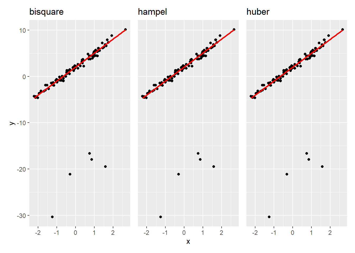

目視では差は殆ど確認できませんが、

list(bisquare = rlm(data$y ~ data$x, method = "M", psi = psi.bisquare, scale.est = "MAD"), hampel = rlm(data$y ~ data$x, method = "M", psi = psi.hampel, scale.est = "MAD"), huber = rlm(data$y ~ data$x, method = "M", psi = psi.huber, scale.est = "MAD"))

$bisquare
Call:
rlm(formula = data$y ~ data$x, psi = psi.bisquare, scale.est = "MAD", 
    method = "M")
Converged in 4 iterations

Coefficients:
(Intercept)      data$x 
    2.01346     3.02080 

Degrees of freedom: 100 total; 98 residual
Scale estimate: 0.498 

$hampel
Call:
rlm(formula = data$y ~ data$x, psi = psi.hampel, scale.est = "MAD", 
    method = "M")
Converged in 3 iterations

Coefficients:
(Intercept)      data$x 
   2.007942    3.023237 

Degrees of freedom: 100 total; 98 residual
Scale estimate: 0.502 

$huber
Call:
rlm(formula = data$y ~ data$x, psi = psi.huber, scale.est = "MAD", 
    method = "M")
Converged in 5 iterations

Coefficients:
(Intercept)      data$x 
   1.967675    3.006463 

Degrees of freedom: 100 total; 98 residual
Scale estimate: 0.543

実際には切片と傾きに差が生じています

それでは300試行のシミュレーションにより、3つの影響関数それぞれのロバスト線形回帰の係数(切片と傾き)を比較します。

fun_simulation <- function(iter, n, nout) {
  formulatxt <- sampledf$y~sampledf$x
  method <- "M"
  maxit <- 100
  scale.est <- "MAD"
  for (iii in seq(iter)) {
    sampledf <- fun_sampledata(seed = iii, n = n, nout = nout)
    # 係数の抽出
    result.rlm.m.mad.bisquare <-
      rlm(formulatxt,
        scale.est = scale.est,
        method = method,
        psi = psi.bisquare,
        maxit = maxit
      )$coef
    result.rlm.m.mad.hampel <-
      rlm(formulatxt,
        scale.est = scale.est,
        method = method,
        psi = psi.hampel,
        maxit = maxit
      )$coef
    result.rlm.m.mad.huber <-
      rlm(formulatxt,
        scale.est = scale.est,
        method = method,
        psi = psi.huber,
        maxit = maxit
      )$coef
    resultdf0 <- rbind(result.rlm.m.mad.bisquare, result.rlm.m.mad.hampel, result.rlm.m.mad.huber) %>%
      t() %>%
      data.frame(check.names = F) %>%
      {
        .$itr <- iii
        .
      }
    if (iii == 1) {
      resultdf_coef <- resultdf0
    } else {
      resultdf_coef <- rbind(resultdf_coef, resultdf0)
    }
  }
  # 切片
  tidydf <- resultdf_coef %>%
    row.names() %>%
    grep("Intercept", .) %>%
    resultdf_coef[., ] %>%
    {
      tidyr::gather(., , , colnames(.)[-4])
    }
  g_coef_intercept <- tidydf %>% ggplot(mapping = aes(x = "", y = value)) +
    geom_boxplot() +
    geom_jitter() +
    facet_wrap(. ~ key, scales = "free_y") +
    theme(axis.title = element_blank()) +
    labs(title = "Intercept") +
    stat_summary(fun = "mean", geom = "point", shape = 23, size = 3, fill = "red")
  # https://r-graphics.org/RECIPE-DISTRIBUTION-BOXPLOT-MEAN.html
  # 傾き
  tidydf <- resultdf_coef %>%
    row.names() %>%
    grep("sampledf", .) %>%
    resultdf_coef[., ] %>%
    {
      tidyr::gather(., , , colnames(.)[-4])
    }
  g_coef_slope <- tidydf %>% ggplot(mapping = aes(x = "", y = value)) +
    geom_boxplot() +
    geom_jitter() +
    facet_wrap(. ~ key, scales = "free_y") +
    theme(axis.title = element_blank()) +
    labs(title = "Slope") +
    stat_summary(fun = "mean", geom = "point", shape = 23, size = 3, fill = "red")
  g_coef_intercept + g_coef_slope + plot_layout(nrow = 2)
}

始めに外れ値を全体の10%とした場合を比較します。

fun_simulation(iter = 300, n = 100, nout = 10)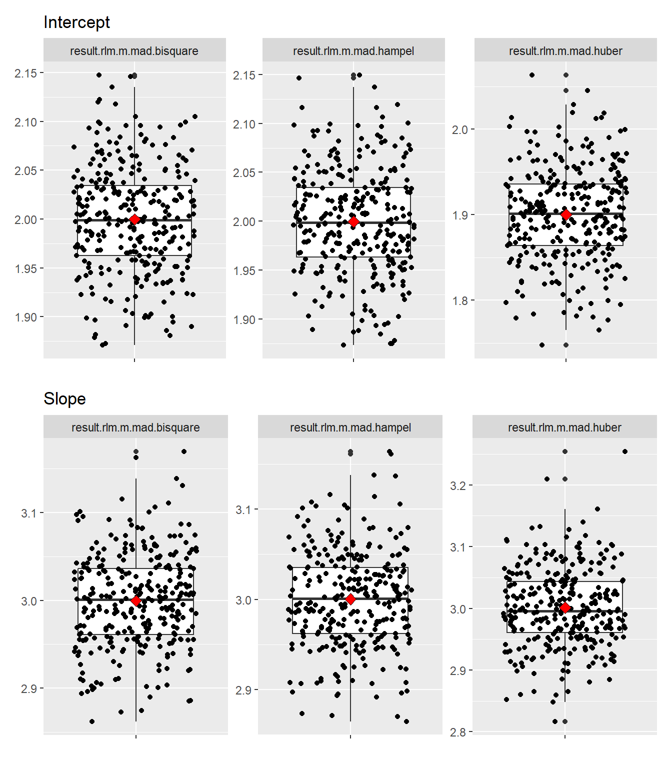

「遠くの外れ値」にも影響を残す huber が他の2つよりも切片が下に引き摺られている事、切片、傾きともに huber は他の2つよりも分散が大きい事を確認できます。

続いて外れ値を全体の20%にした場合です。

fun_simulation(iter = 300, n = 100, nout = 20)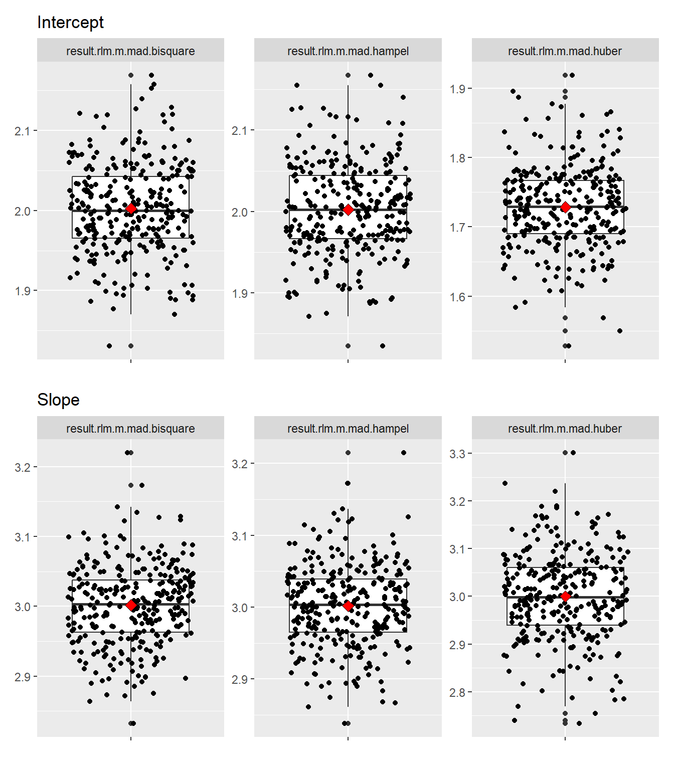

huber では、外れ値を10%とした場合よりもさらに切片が下に引き摺られている事、他の2つの影響関数よりも切片、傾きともに分散が大きいことを確認できます。

以上です。