
ロバスト線形回帰を扱うRの関数 rlm {MASS} について、引数 method を M推定 とした場合と、MM推定 とした場合それぞれの結果をシミュレーションで比較します。
本ポストは以下の資料を参照引用しています。
- https://www.stat.go.jp/training/2kenkyu/ihou/76/pdf/2-2-767.pdf
- https://www.st.nanzan-u.ac.jp/info/gr-thesis/ms/2004/kimura/01mm029.pdf
- https://stat.ethz.ch/R-manual/R-devel/library/MASS/html/lqs.html
始めに外れ値のあるサンプルデータを生成する関数を作成します。
なお、外れ値は全て「意図的に大きな外れ」とし、かつ回帰直線を「下方向に引っ張る」値とします。
library(dplyr)
fun_sampledata <- function(seed, n, nout) {
  set.seed(seed)

  # 真のモデル: y = 2 + 3x + ε
  x <- rnorm(n)
  y_true <- 2 + 3 * x
  y <- y_true + rnorm(n, sd = 0.5)

  # 外れ値追加
  id_out <- sample(x = seq(n), size = nout, replace = F)
  y[id_out] <- y_true[id_out] + runif(n = nout, min = -30, max = -20)

  data <- data.frame(x = x, y = y)
  return(data)
}
サンプルサイズは100点。うち5点(全体の5%)を外れ値としたサンプルです。
seed <- 20250324
n <- 100
nout <- 5 # 外れ値数
data <- fun_sampledata(seed = seed, n = n, nout = nout)
glimpse(data)
Rows: 100
Columns: 2
$ x <dbl> -1.12431561, 1.11381324, 2.26219692, -0.45547576, 0.46294328, -0.128…
$ y <dbl> -1.87119307, 5.75566928, 8.14380579, 0.75527946, 3.79927589, 1.23719…外れ度合い をチャートで確認します。
library(ggplot2)
ggplot(data = data, mapping = aes(x = x, y = y)) +
  geom_point()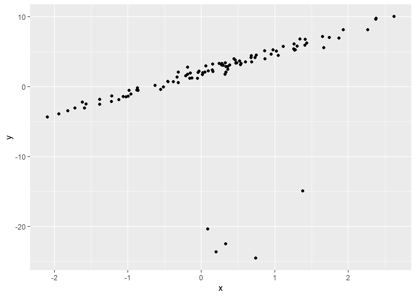
作成したサンプルデータについて、MM推定 および M推定 の結果をチャートで比較します。
library(MASS)
library(patchwork)
g1 <- ggplot(data = data, mapping = aes(x = x, y = y)) +
  geom_point() +
  geom_smooth(method = "lm", se = F, color = "blue") +
  geom_smooth(method = "rlm", se = F, color = "red", method.args = list(method = "MM")) +
  labs(title = "青色:lm,赤色:rlm(MM)")
g2 <- ggplot(data = data, mapping = aes(x = x, y = y)) +
  geom_point() +
  geom_smooth(method = "lm", se = F, color = "blue") +
  geom_smooth(method = "rlm", se = F, color = "red", method.args = list(method = "M", psi = psi.bisquare, scale.est = "MAD")) +
  labs(title = "青色:lm,赤色:rlm(M)")
g1 + g2 + plot_layout(axes = "collect")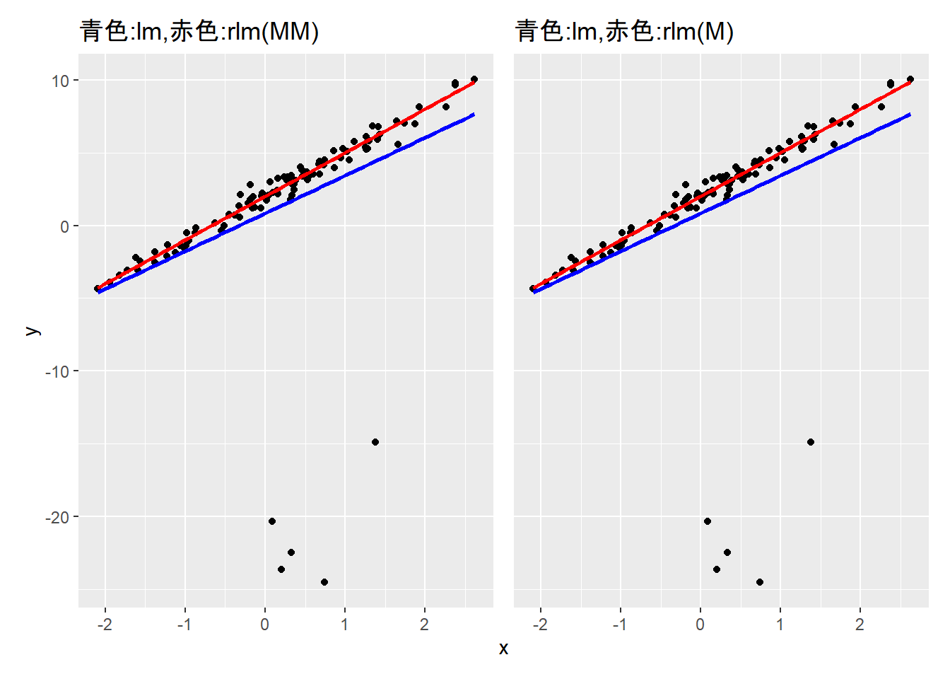
通常の線形回帰(lm)では切片が下側に引き摺られていることを確認できると同時に、目視では MM推定 と M推定 に差はほぼ見られません。
それでは300試行のシミュレーションにより、通常の線形回帰、MM推定 によるロバスト回帰、M推定 によるロバスト回帰それぞれの 切片 と 傾き を比較します。
fun_simulation <- function(iter, n, nout, object) {
  for (iii in seq(iter)) {
    sampledf <- fun_sampledata(seed = iii, n = n, nout = nout)
    result.lm <- lm(sampledf$y ~ sampledf$x)$coef
    result.rlm.m <- rlm(sampledf$y ~ sampledf$x, , method = "M", scale.est = "MAD", psi = psi.bisquare, maxit = 100)$coef
    result.rlm.mm <- rlm(sampledf$y ~ sampledf$x, , method = "MM", maxit = 100)$coef
    resultdf0 <- rbind(result.lm, result.rlm.m, result.rlm.mm) %>%
      t() %>%
      data.frame(check.names = F) %>%
      {
        .$itr <- iii
        .
      }
    if (iii == 1) {
      resultdf <- resultdf0
    } else {
      resultdf <- rbind(resultdf, resultdf0)
    }
  }
  tidydf <- resultdf %>%
    row.names() %>%
    grep(object, .) %>%
    resultdf[., ] %>%
    {
      tidyr::gather(., , , colnames(.)[-4])
    }
  tidydf %>% ggplot(mapping = aes(x = "", y = value)) +
    geom_boxplot() +
    geom_jitter() +
    facet_wrap(. ~ key, scales = "free_y") +
    theme(axis.title = element_blank())
}
始めに外れ値を全体の10%とした場合の切片を比較します。
fun_simulation(iter = 300, n = 100, nout = 10, object = "Intercept")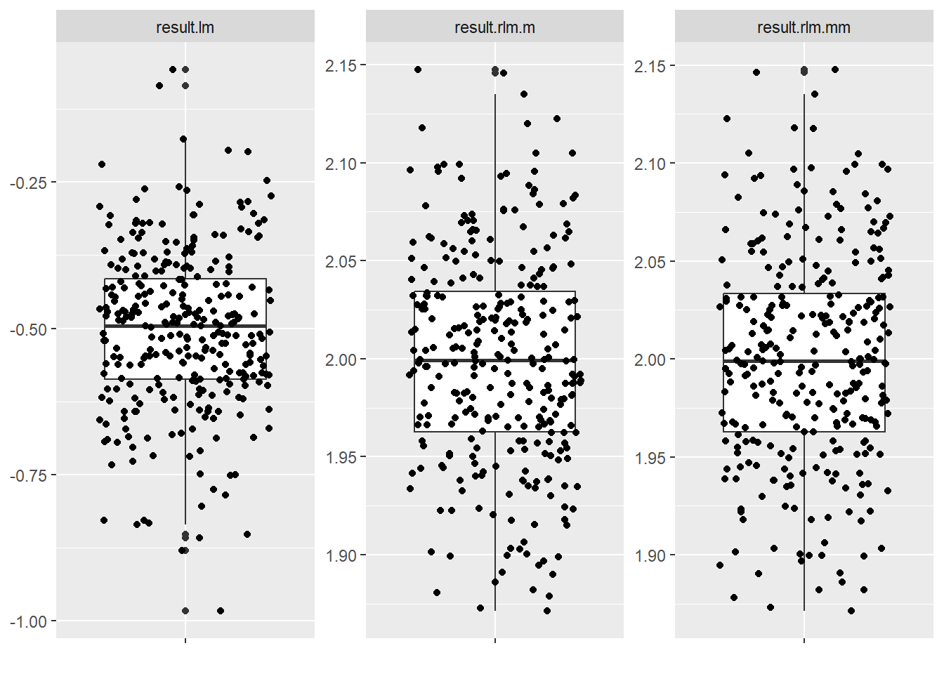
通常の線形回帰(result.lm)では切片の中央値は -0.50 程度まで引き摺られていますが、ロバスト線形回帰では M推定(result.rlm.m) も MM推定(result.rlm.mm)も 2.0 程度にあり、かつ 1.85 から 2.15 の間に殆どの結果が収まっています。
続いて外れ値を全体の30%にした場合です。
fun_simulation(iter = 300, n = 100, nout = 30, object = "Intercept")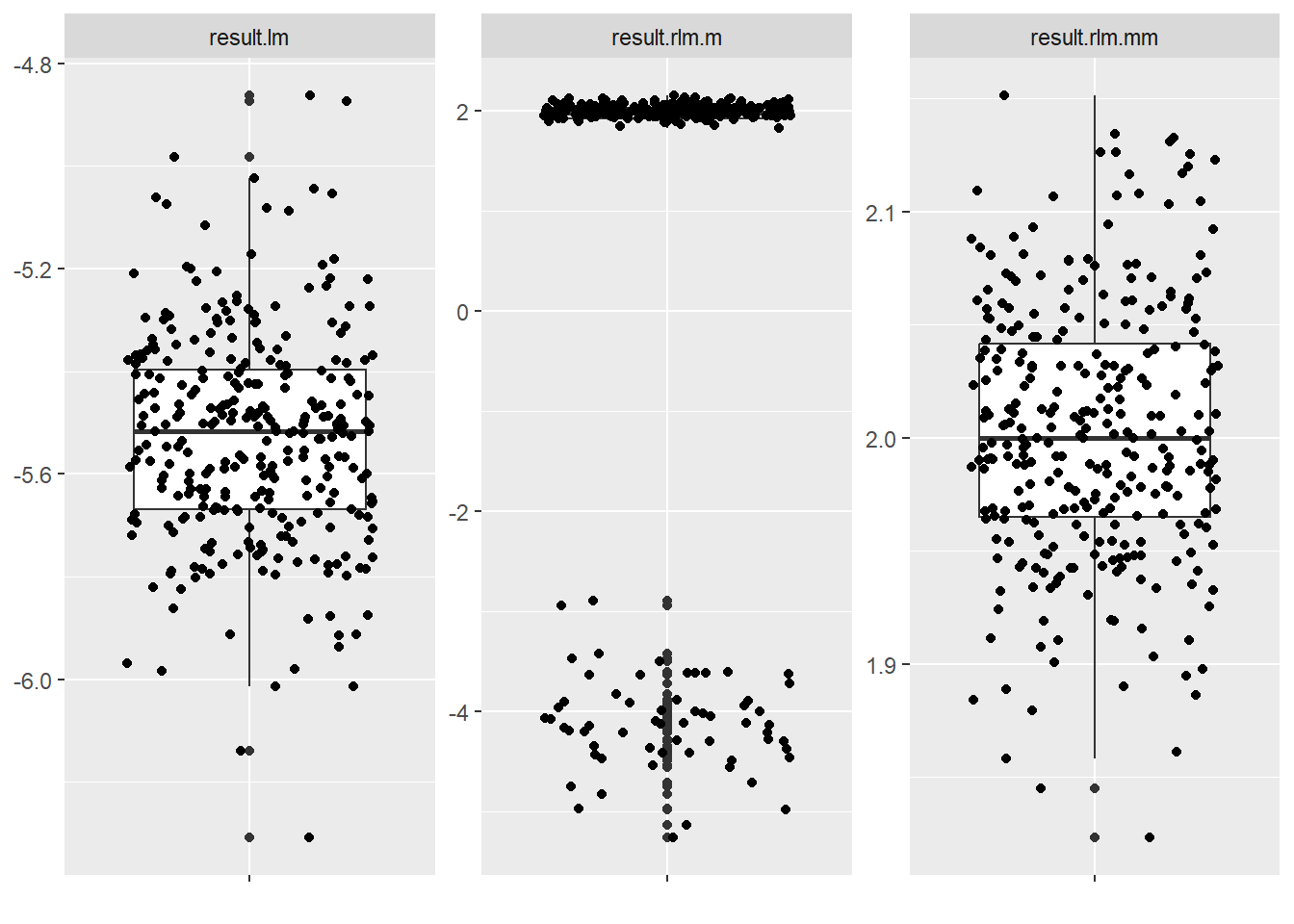
通常の線形回帰では切片の中央値は -5.5 程度まで引き摺られています。
M推定では切片の中央値は 2.0 程度ですが -3.0 から -5.0 の間まで引き摺られている結果もあり、MM推定 では中央値は 2.0 程度、試行全体としても、外れ値を全体の10%とした場合と同様に、1.85 から 2.15 の間に殆どの結果が収まっています。
続いて傾きを比較します
外れ値を全体の10%とした場合です。
fun_simulation(iter = 300, n = 100, nout = 10, object = "sampledf")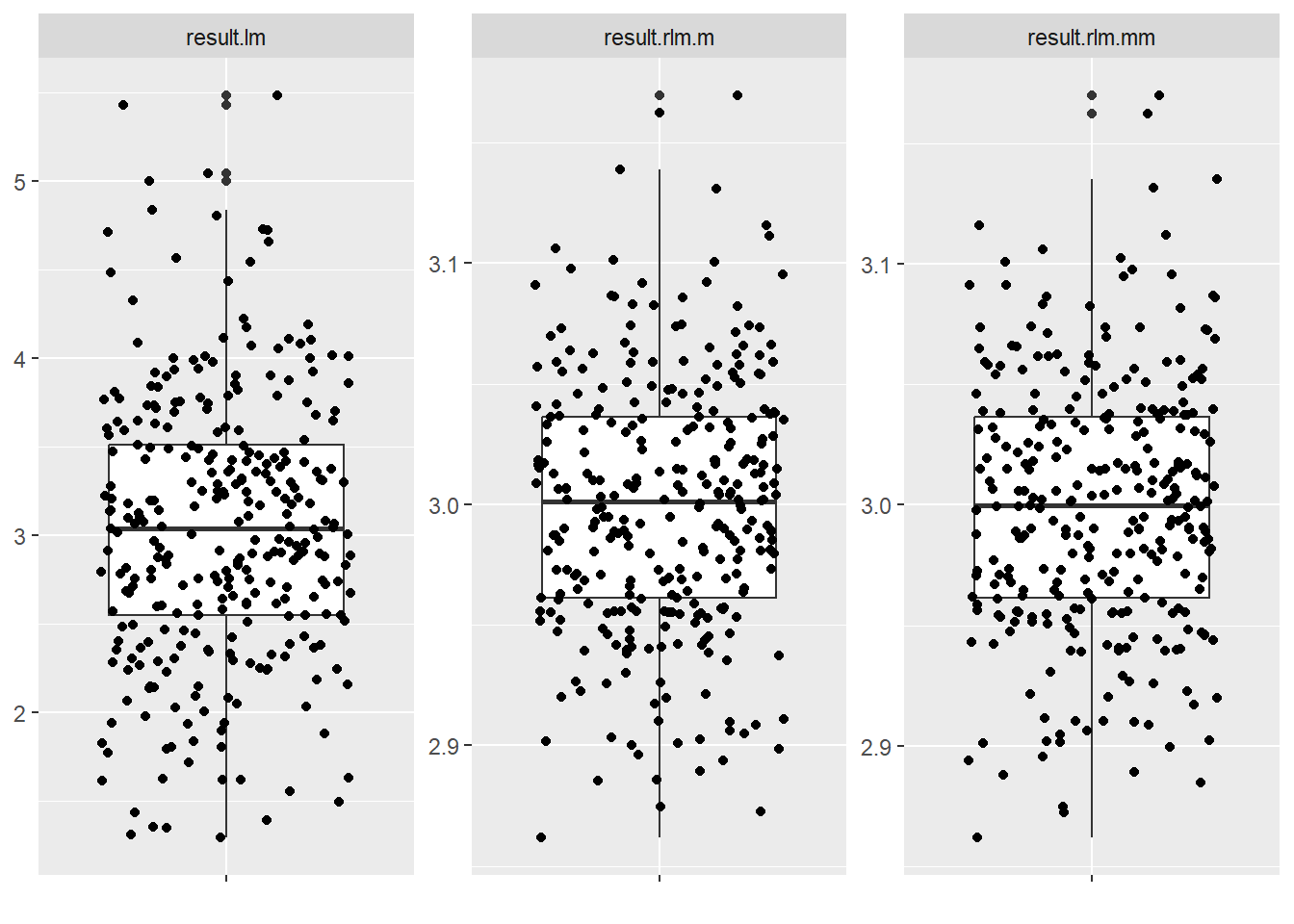
いずれの回帰の場合も傾きの中央値は 3.0 程度の結果ですが、通常の線形回帰は2つのロバスト線形回帰よりも結果の分散が大きいようです。
続いて外れ値を全体の30%にした場合です。
fun_simulation(iter = 300, n = 100, nout = 30, object = "sampledf")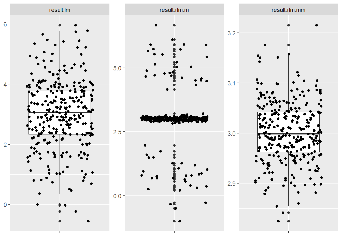
こちらも傾きの中央値は3つの回帰いずれも 3.0 程度の結果ですが、通常の線形回帰も M推定 も傾きの推定値のバラつきが大きく、しかし、MM推定 では 2.8 から 3.2 の間に殆どが収まっています。
最後にコメントを挿入しました関数 rlm.default のコードを記します。
# 引数:
#   x: 説明変数の行列(デザイン行列)。各列が変数を表し、各行が観測値を表す。
#   y: 応答変数のベクトル。観測された応答変数の値。
#   weights: 観測値に対する重みベクトル。デフォルトでは使用されない。
#   w: IRLS(反復重み付け最小二乗法)で使用する初期重み。デフォルトは1のベクトル。
#   init: 初期推定方法。"ls"(最小二乗法)または"lts"(最小トリミング二乗法)が選択可能。
#   psi: ロバスト推定に使用するψ関数(影響関数)。デフォルトはHuber関数。
#   scale.est: スケール推定方法。"MAD"(中央絶対偏差)、"Huber"、"proposal 2"のいずれか。
#   k2: ψ関数のチューニング定数。Huber関数では1.345が標準値。
#   method: 推定方法。"M"(M推定)または"MM"(MM推定)。
#   wt.method: 重みの計算方法。"inv.var"(分散の逆数)または"case"(ケースごとの重み)。
#   maxit: IRLSの最大反復回数。デフォルトは20。
#   acc: 収束判定の精度。デフォルトは1e-04。
#   test.vec: 収束テストに使用する基準。"resid"(残差)、"coef"(係数)、"w"(重み)など。
#   lqs.control: lqs(ロバスト回帰)の制御パラメータ。
function(x, y, weights, ..., w = rep(1, nrow(x)), init = "ls",
         psi = psi.huber, scale.est = c("MAD", "Huber", "proposal 2"),
         k2 = 1.345, method = c("M", "MM"), wt.method = c("inv.var", "case"),
         maxit = 20, acc = 1e-04, test.vec = "resid", lqs.control = NULL) {
  # IRLS収束判定のための差分計算関数
  # 数学的意味: 古い推定値(old)と新しい推定値(new)のユークリッド距離を正規化。
  # 具体的には、差の二乗和の平方根を、古い値の二乗和(ゼロ除算回避のため1e-20と比較)で割る。
  irls.delta <- function(old, new) sqrt(sum((old - new)^2) / max(1e-20, sum(old^2)))

  # IRLSにおける重み付き残差の最大絶対値を計算する関数
  # 数学的意味: 重み付き残差(r * sqrt(w))とデザイン行列(x)の内積の絶対値の最大値を、
  # 重み付き残差の二乗和の平方根で正規化。これにより、収束判定に使用するスケール調整された指標を計算。
  irls.rrxwr <- function(x, w, r) {
    w <- sqrt(w) # 重みの平方根を取る(重みのスケール調整)
    max(abs((matrix(r * w, 1L, length(r)) %*% x) / sqrt(matrix(w, 1L, length(r)) %*% (x^2)))) / sqrt(sum(w * r^2))
  }

  # 重み付き中央絶対偏差(Weighted MAD)を計算する関数
  # 数学的意味: ロバストなスケール推定のために、観測値の絶対値の中央値を重み付きで求める。
  # 具体的には、重みの累積和が0.5を超える点を補間し、0.6745でスケール調整(正規分布の仮定)。
  wmad <- function(x, w) {
    o <- sort.list(abs(x)) # 絶対値の昇順に並べ替えたインデックスを取得
    x <- abs(x)[o] # 絶対値をソート
    w <- w[o] # 重みも同じ順序にソート
    p <- cumsum(w) / sum(w) # 重みの累積分布を計算
    n <- sum(p < 0.5) # 累積分布が0.5未満の観測点数
    if (p[n + 1L] > 0.5) {
      x[n + 1L] / 0.6745
    } # 0.5を超える最初の点を使用し、スケール調整
    else {
      (x[n + 1L] + x[n + 2L]) / (2 * 0.6745)
    } # 0.5を挟む2点の平均を使用
  }

  # 引数のマッチング
  method <- match.arg(method) # method引数を"M"または"MM"に制限
  wt.method <- match.arg(wt.method) # wt.method引数を"inv.var"または"case"に制限

  # デザイン行列の名前処理
  nmx <- deparse(substitute(x)) # xの変数名を文字列として取得
  if (is.null(dim(x))) { # xがベクトルの場合、行列に変換
    x <- as.matrix(x)
    colnames(x) <- nmx
  } else {
    x <- as.matrix(x)
  }
  if (is.null(colnames(x))) { # 列名がない場合、デフォルト名を付与
    colnames(x) <- paste("X", seq(ncol(x)), sep = "")
  }

  # デザイン行列のランクチェック
  # 数学的意味: xの列ランクが列数未満の場合、特異行列となり逆行列が存在しないためエラー。
  if (qr(x)$rank < ncol(x)) {
    stop("'x' is singular: singular fits are not implemented in 'rlm'")
  }

  # 収束テストベクトルの有効性チェック
  if (!(any(test.vec == c("resid", "coef", "w", "NULL")) || is.null(test.vec))) {
    stop("invalid 'test.vec'")
  }

  # データのコピー
  xx <- x
  yy <- y

  # 重みの処理
  if (!missing(weights)) { # weightsが指定されている場合
    if (length(weights) != nrow(x)) {
      stop("length of 'weights' must equal number of observations")
    }
    if (any(weights < 0)) {
      stop("negative 'weights' value")
    }
    if (wt.method == "inv.var") { # 分散の逆数に基づく重み付け
      fac <- sqrt(weights) # 重みの平方根を計算
      y <- y * fac # 応答変数をスケール調整
      x <- x * fac # 説明変数をスケール調整
      wt <- NULL
    } else { # ケースごとの重み
      w <- w * weights # IRLSの重みに観測重みを乗じる
      wt <- weights
    }
  } else {
    wt <- NULL
  }

  # M推定の場合
  if (method == "M") {
    scale.est <- match.arg(scale.est) # スケール推定方法を制限
    if (!is.function(psi)) { # psiが関数でない場合、名前から関数を取得
      psi <- get(psi, mode = "function")
    }
    arguments <- list(...) # その他の引数を取得
    if (length(arguments)) { # 追加引数があればpsi関数に適用
      pm <- pmatch(names(arguments), names(formals(psi)), nomatch = 0L)
      if (any(pm == 0L)) {
        warning("some of ... do not match")
      }
      pm <- names(arguments)[pm > 0L]
      formals(psi)[pm] <- unlist(arguments[pm])
    }

    # 初期推定値の計算
    if (is.character(init)) {
      temp <- if (init == "ls") { # 最小二乗法による初期化
        lm.wfit(x, y, w, method = "qr")
      } else if (init == "lts") { # 最小トリミング二乗法による初期化
        if (is.null(lqs.control)) {
          lqs.control <- list(nsamp = 200L)
        }
        do.call("lqs", c(list(x, y, intercept = FALSE), lqs.control))
      } else {
        stop("'init' method is unknown")
      }
      coef <- temp$coefficients # 回帰係数の初期値
      resid <- temp$residuals # 残差の初期値
    } else {
      if (is.list(init)) {
        coef <- init$coef
      } else {
        coef <- init
      }
      resid <- drop(y - x %*% coef) # 初期係数に基づく残差
    }
  }
  # MM推定の場合
  else if (method == "MM") {
    scale.est <- "MM" # MM推定ではスケールは固定
    temp <- do.call("lqs", c(list(x, y, intercept = FALSE, method = "S", k0 = 1.548), lqs.control))
    coef <- temp$coefficients # S推定による初期係数
    resid <- temp$residuals # 初期残差
    psi <- psi.bisquare # MM推定ではbi-square関数を使用
    if (length(arguments <- list(...))) {
      if (match("c", names(arguments), nomatch = 0L)) {
        c0 <- arguments$c
        if (c0 > 1.548) {
          formals(psi)$c <- c0
        } # bi-squareのチューニング定数を調整
        else {
          warning("'c' must be at least 1.548 and has been ignored")
        }
      }
    }
    scale <- temp$scale # S推定によるスケール
  } else {
    stop("'method' is unknown")
  }

  # IRLSの初期化
  done <- FALSE # 収束フラグ
  conv <- NULL # 収束履歴
  n1 <- (if (is.null(wt)) nrow(x) else sum(wt)) - ncol(x) # 自由度(観測数 - 変数数)

  # ψ関数の効率性に関連する定数の計算
  # 数学的意味: Huber関数のチューニング定数k2に基づき、期待されるロバスト性を計算。
  # theta: 正規分布でのk2に基づく効率性、gamma: 分散の調整係数。
  theta <- 2 * pnorm(k2) - 1
  gamma <- theta + k2^2 * (1 - theta) - 2 * k2 * dnorm(k2)

  # 初期スケールの計算
  if (scale.est != "MM") {
    scale <- if (is.null(wt)) mad(resid, 0) else wmad(resid, wt)
  }

  # IRLS反復ループ
  for (iiter in 1L:maxit) {
    if (!is.null(test.vec)) {
      testpv <- get(test.vec)
    } # 収束テスト用の前回値を保存

    # スケールの更新
    if (scale.est != "MM") {
      scale <- if (scale.est == "MAD") {
        if (is.null(wt)) median(abs(resid)) / 0.6745 else wmad(resid, wt)
      } else if (is.null(wt)) {
        sqrt(sum(pmin(resid^2, (k2 * scale)^2)) / (n1 * gamma))
      } else {
        sqrt(sum(wt * pmin(resid^2, (k2 * scale)^2)) / (n1 * gamma))
      }
      if (scale == 0) { # スケールが0の場合、収束とみなす
        done <- TRUE
        break
      }
    }

    # 重みの計算
    w <- psi(resid / scale) # 残差をスケールで割った値にψ関数を適用
    if (!is.null(wt)) {
      w <- w * weights
    } # 観測重みを適用

    # 重み付き最小二乗法で係数を更新
    temp <- lm.wfit(x, y, w, method = "qr")
    coef <- temp$coefficients
    resid <- temp$residuals

    # 収束判定
    if (!is.null(test.vec)) {
      convi <- irls.delta(testpv, get(test.vec))
    } else {
      convi <- irls.rrxwr(x, w, resid)
    }
    conv <- c(conv, convi)
    done <- (convi <= acc) # 収束条件を満たせば終了
    if (done) {
      break
    }
  }

  # 収束しなかった場合の警告
  if (!done) {
    warning(gettextf("'rlm' failed to converge in %d steps", maxit), domain = NA)
  }

  # 予測値の計算
  fitted <- drop(xx %*% coef)

  # 呼び出し情報の保存
  cl <- match.call()
  cl[[1L]] <- as.name("rlm")

  # 結果のリストを作成
  fit <- list(
    coefficients = coef, residuals = yy - fitted,
    wresid = resid, effects = temp$effects, rank = temp$rank,
    fitted.values = fitted, assign = temp$assign, qr = temp$qr,
    df.residual = NA, w = w, s = scale, psi = psi, k2 = k2,
    weights = if (!missing(weights)) weights, conv = conv,
    converged = done, x = xx, call = cl
  )
  class(fit) <- c("rlm", "lm") # クラスを指定
  fit # 結果を返す
}確率誤差: probable errorの訳で,〈確からしい誤差〉ともいう。多数の測定値から最も確からしい値を推定したとき,前者と後者の差(つまり誤差)の絶対値がrより小さい測定値と大きい測定値が同数であるとき,rを確率誤差という。誤差が正規分布に従うときはrは標準偏差の0.6745倍に等しいので,測定値から求めた標準誤差(誤差の2乗の平均値の平方根)の0.6745倍を確率誤差とする。これが小さいほど測定の精度が高く,測定から得た最も確からしい値のあとに±をつけて表示する。なお,確率誤差は現在では一般に使われておらず,標準偏差を用いる。 出所:https://kotobank.jp/word/%E7%A2%BA%E7%8E%87%E8%AA%A4%E5%B7%AE-43859
以上です。