Rで切片と傾きの検定

時系列データを任意の時点で2つに分割した際に、分割前後の線形回帰の結果に有意な差があるか否かの検定です。

なお、関数 lm {stats} の交差項を利用せずに分散共分散により検定する方法は、Rで統計的仮説検定:共分散分析を参照してください。

始めに切片は同一、傾きは異なるサンプルデータを作成します。サンプルサイズは100点とし、50点目で傾きのみ変化させます。

library(dplyr)
library(ggplot2)
fun_generate_sample <- function(seed, n, split_point, b0_period1, b0_period2, b1_period1, b1_period2) {
  set.seed(seed)
  time <- seq(n)
  y <- numeric(length = n)
  id_perion1 <- seq(n) %>% head(split_point)
  id_perion2 <- seq(n) %>% tail(split_point)
  y[id_perion1] <- b0_period1 + b1_period1 * time[seq(n) %>% head(split_point)] + rnorm(length(id_perion1))
  y[id_perion2] <- b0_period2 + b1_period2 * time[seq(n) %>% tail(split_point)] + rnorm(length(id_perion2))
  data <- data.frame(time = time, y = y)
  data$period[id_perion1] <- "period1"
  data$period[id_perion2] <- "period2"
  data$period <- data$period %>% as.factor()
  return(data)
}
data <- fun_generate_sample(seed = 20250315, n = 100, split_point = 50, b0_period1 = 2, b0_period2 = 2, b1_period1 = 2, b1_period2 = 4)
ggplot(data = data, mapping = aes(x = time, y = y, colour = period)) +
  geom_point()

period1 と period2 で傾きおよび切片に有意な差が生じているか検定します。有意水準は5%とします。

なお、説明変数 periodperiod2 はピリオドの主効果(切片の差を捉える部分)であり、具体的には、基準ピリオド period1 からの切片の差を表します。

また、説明変数 time:periodperiod2 は時間とピリオドの交互作用効果(傾きの差を捉える部分)であり、具体的には、基準ピリオド period1 からの傾きの差を表します。

lm(y ~ time * period, data = data) %>% summary()


Call:
lm(formula = y ~ time * period, data = data)

Residuals:
     Min       1Q   Median       3Q      Max 
-2.53063 -0.61068  0.00182  0.74349  1.79597 

Coefficients:
                    Estimate Std. Error t value Pr(>|t|)    
(Intercept)         2.356380   0.264375   8.913 3.21e-14 ***
time                1.985696   0.009023 220.071  < 2e-16 ***
periodperiod2      -0.968878   0.742246  -1.305    0.195    
time:periodperiod2  2.021544   0.012760 158.423  < 2e-16 ***
---
Signif. codes:  0 '***' 0.001 '**' 0.01 '*' 0.05 '.' 0.1 ' ' 1

Residual standard error: 0.9207 on 96 degrees of freedom
Multiple R-squared:      1, Adjusted R-squared:      1 
F-statistic: 7.009e+05 on 3 and 96 DF,  p-value: < 2.2e-16

結果のうち、

(Intercept) は基準ピリオドである period1 の切片の推定値です。
time は基準ピリオドである period1 の傾きの推定値です。
periodperiod2 は period2 の切片が period1 の切片と比較してどれだけ異なるかを表す係数です。p値は0.195と95%信頼区間がゼロを跨ぎます。
time:periodperiod2 は period2 の傾きが period1 の傾きと比較してどれだけ異なるかを表す係数です。p値は2e-16と95%信頼区間はゼロを跨ぎません。

periodperiod2 は棄却されず time:periodperiod2 棄却されますので、切片が同一との仮説は棄却されず、傾きは同一との仮説は棄却されます。

続いて傾きは同一、切片が異なるサンプルを確認します。

data <- fun_generate_sample(seed = 20250315, n = 100, split_point = 50, b0_period1 = 10, b0_period2 = 2, b1_period1 = 2, b1_period2 = 2)
ggplot(data = data, mapping = aes(x = time, y = y, colour = period)) +
  geom_point()
lm(y ~ time * period, data = data) %>% summary()


Call:
lm(formula = y ~ time * period, data = data)

Residuals:
     Min       1Q   Median       3Q      Max 
-2.53063 -0.61068  0.00182  0.74349  1.79597 

Coefficients:
                    Estimate Std. Error t value Pr(>|t|)    
(Intercept)        10.356380   0.264375  39.173   <2e-16 ***
time                1.985696   0.009023 220.071   <2e-16 ***
periodperiod2      -8.968878   0.742246 -12.083   <2e-16 ***
time:periodperiod2  0.021544   0.012760   1.688   0.0946 .  
---
Signif. codes:  0 '***' 0.001 '**' 0.01 '*' 0.05 '.' 0.1 ' ' 1

Residual standard error: 0.9207 on 96 degrees of freedom
Multiple R-squared:  0.9997,    Adjusted R-squared:  0.9997 
F-statistic: 1.157e+05 on 3 and 96 DF,  p-value: < 2.2e-16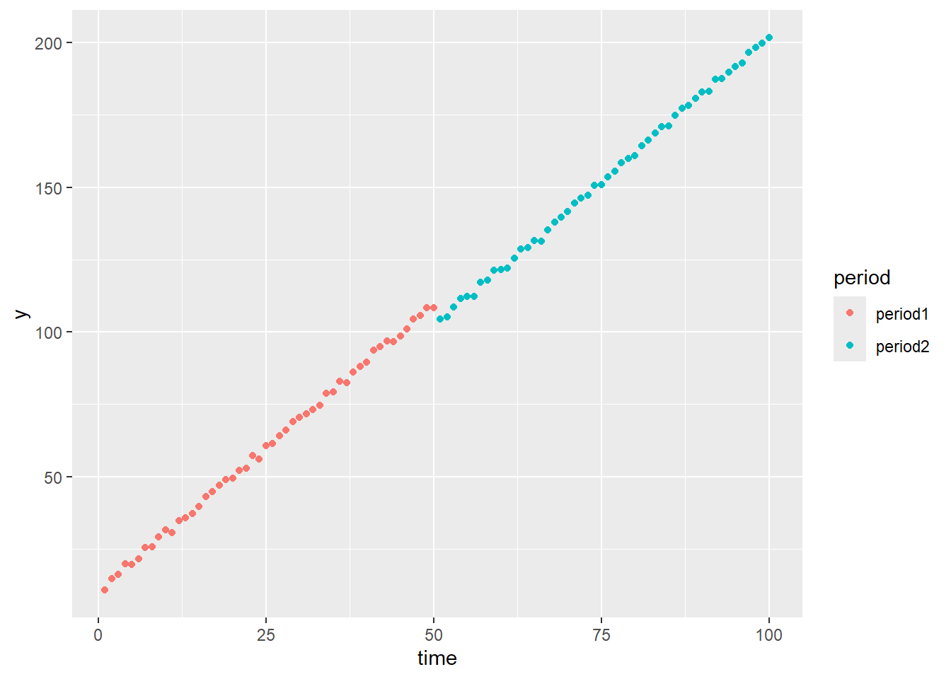

切片は同一との仮説は棄却され、傾きは同一との仮説は棄却されません。

傾きも切片も異なるサンプルを確認します。

data <- fun_generate_sample(seed = 20250315, n = 100, split_point = 50, b0_period1 = 4, b0_period2 = 2, b1_period1 = 2, b1_period2 = 4)
ggplot(data = data, mapping = aes(x = time, y = y, colour = period)) +
  geom_point()
lm(y ~ time * period, data = data) %>% summary()


Call:
lm(formula = y ~ time * period, data = data)

Residuals:
     Min       1Q   Median       3Q      Max 
-2.53063 -0.61068  0.00182  0.74349  1.79597 

Coefficients:
                    Estimate Std. Error t value Pr(>|t|)    
(Intercept)         4.356380   0.264375   16.48  < 2e-16 ***
time                1.985696   0.009023  220.07  < 2e-16 ***
periodperiod2      -2.968878   0.742246   -4.00 0.000125 ***
time:periodperiod2  2.021544   0.012760  158.42  < 2e-16 ***
---
Signif. codes:  0 '***' 0.001 '**' 0.01 '*' 0.05 '.' 0.1 ' ' 1

Residual standard error: 0.9207 on 96 degrees of freedom
Multiple R-squared:      1, Adjusted R-squared:      1 
F-statistic: 6.911e+05 on 3 and 96 DF,  p-value: < 2.2e-16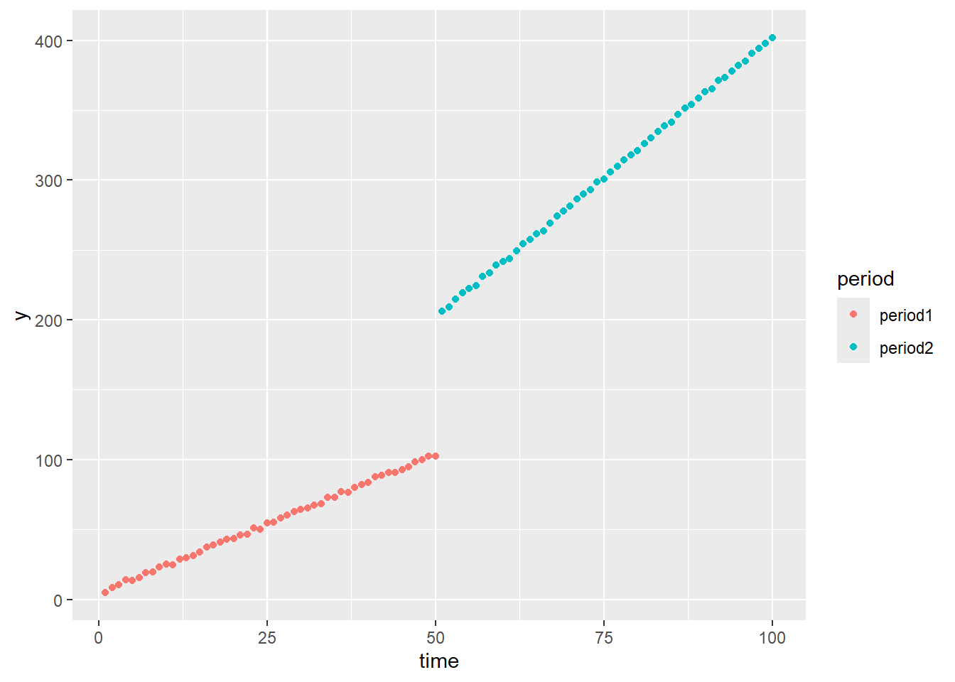

切片、傾きとも両ピリオドで同一との仮説は棄却されます。

最後に傾きも切片も同一のサンプルで確認します。

data <- fun_generate_sample(seed = 20250315, n = 100, split_point = 50, b0_period1 = 4, b0_period2 = 4, b1_period1 = 4, b1_period2 = 4)
ggplot(data = data, mapping = aes(x = time, y = y, colour = period)) +
  geom_point()
lm(y ~ time * period, data = data) %>% summary()


Call:
lm(formula = y ~ time * period, data = data)

Residuals:
     Min       1Q   Median       3Q      Max 
-2.53063 -0.61068  0.00182  0.74349  1.79597 

Coefficients:
                    Estimate Std. Error t value Pr(>|t|)    
(Intercept)         4.356380   0.264375  16.478   <2e-16 ***
time                3.985696   0.009023 441.728   <2e-16 ***
periodperiod2      -0.968878   0.742246  -1.305   0.1949    
time:periodperiod2  0.021544   0.012760   1.688   0.0946 .  
---
Signif. codes:  0 '***' 0.001 '**' 0.01 '*' 0.05 '.' 0.1 ' ' 1

Residual standard error: 0.9207 on 96 degrees of freedom
Multiple R-squared:  0.9999,    Adjusted R-squared:  0.9999 
F-statistic: 5.238e+05 on 3 and 96 DF,  p-value: < 2.2e-16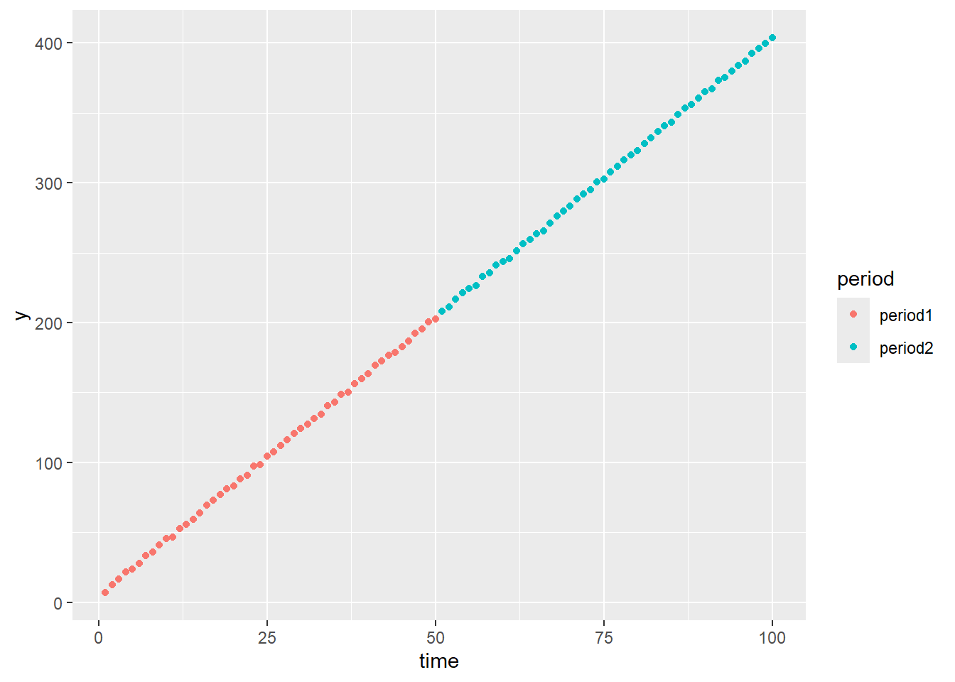

切片、傾きとも両ピリオドで同一との仮説は棄却されません。

以上です。