
Rで 差分の差分法(Difference-in-Differences: DID) を試みます。
始めにサンプルデータを作成します。
library(tidyverse)

# パラメータ設定
n_per_group <- 100 # 各グループの個体数 (サンプルサイズ)
time_points <- 2 # 時間点 (0: 介入前, 1: 介入後)
baseline_mean <- 10 # 介入前の平均アウトカム(対照群)
time_trend_effect <- 2 # 時間経過による共通の効果(両群に影響)
treatment_effect <- 6.5 # 介入(処置)の効果(処置群の介入後にのみ影響)
sd_noise <- 2 # 個体差や測定誤差などのノイズの標準偏差

# サンプルデータを格納するデータフレームを作成
df <- expand.grid(
  id = 1:(n_per_group * 2), # 個体ID
  time = 0:(time_points - 1) # 時間 (0: 前, 1: 後)
) %>%
  as_tibble() %>%
  arrange(id, time)

# 処置群か対照群かを割り当てる (idが101以上を処置群とする)
df <- df %>%
  mutate(
    treatment_group = ifelse(id > n_per_group, 1, 0), # 0: 対照群, 1: 処置群
    # time_post = time # timeが0/1なので time_post = time と同じ。
  )
一旦、データフレームを確認します。
head(df)# A tibble: 6 × 3
id time treatment_group
<int> <int> <dbl>
1 1 0 0
2 1 1 0
3 2 0 0
4 2 1 0
5 3 0 0
6 3 1 0続けます。
seed <- 20250420
set.seed(seed)

# アウトカム変数の生成
# 介入前のベースラインのアウトカムを生成(個体差を含む)
baseline_outcome <- rnorm(n_per_group * 2, mean = baseline_mean, sd = sd_noise)
df <- df %>%
  mutate(
    # 各個体のベースラインアウトカムを対応させる
    baseline_y = baseline_outcome[id],
    # 時間経過効果と処置効果、ノイズを加味してアウトカムを計算
    outcome = baseline_y + # ベースライン
      time * time_trend_effect + # 時間トレンド効果 (両群共通)
      treatment_group * time * treatment_effect + # 処置効果 (処置群のtime=1のみ)
      rnorm(n(), mean = 0, sd = sd_noise) # 各時点での追加ノイズ
  ) %>%
  # 不要な中間変数を削除
  select(-baseline_y)
作成しましたサンプルデータを確認します。
head(df)
str(df)
# A tibble: 6 × 4
id time treatment_group outcome
<int> <int> <dbl> <dbl>
1 1 0 0 12.5
2 1 1 0 14.2
3 2 0 0 8.07
4 2 1 0 7.53
5 3 0 0 11.2
6 3 1 0 14.6
tibble [400 × 4] (S3: tbl_df/tbl/data.frame)
$ id : int [1:400] 1 1 2 2 3 3 4 4 5 5 ...
$ time : int [1:400] 0 1 0 1 0 1 0 1 0 1 ...
$ treatment_group: num [1:400] 0 0 0 0 0 0 0 0 0 0 ...
$ outcome : num [1:400] 12.47 14.22 8.07 7.53 11.22 ...
- attr(*, "out.attrs")=List of 2
..$ dim : Named int [1:2] 200 2
.. ..- attr(*, "names")= chr [1:2] "id" "time"
..$ dimnames:List of 2
.. ..$ id : chr [1:200] "id= 1" "id= 2" "id= 3" "id= 4" ...
.. ..$ time: chr [1:2] "time=0" "time=1"グループ別・時期別の平均アウトカムを求めます。
(summary_df <- df %>%
  group_by(treatment_group, time) %>%
  summarise(mean_outcome = mean(outcome), .groups = "drop")) # .groups='drop'でgroup化を解除しています
# A tibble: 4 × 3
treatment_group time mean_outcome
<dbl> <int> <dbl>
1 0 0 10.2
2 0 1 12.0
3 1 0 10.5
4 1 1 18.8サンプルデータを可視化し、平均値の推移を確認します。
plot_trends <- function() {
  ggplot(summary_df, aes(
    x = factor(time), y = mean_outcome,
    color = factor(treatment_group), group = factor(treatment_group)
  )) +
    geom_line(linewidth = 1) +
    geom_point(size = 3) +
    # 介入のタイミングを示す垂直線
    geom_vline(xintercept = 1.5, linetype = "dashed", color = "grey50") +
    annotate("text", x = 1.5, y = max(summary_df$mean_outcome), label = "介入", hjust = -0.1, vjust = 1, color = "grey50") +
    scale_x_discrete(labels = c("0" = "介入前", "1" = "介入後")) +
    scale_color_manual(
      values = c("0" = "blue", "1" = "red"),
      labels = c("0" = "対照群 (Control)", "1" = "処置群 (Treatment)"),
      name = "グループ"
    ) +
    labs(
      title = "グループ別のアウトカム平均値の推移",
      subtitle = "差分の差分法 (DID) の視覚化",
      x = "時期",
      y = "アウトカム平均値"
    ) +
    theme_minimal()
}
plot_trends()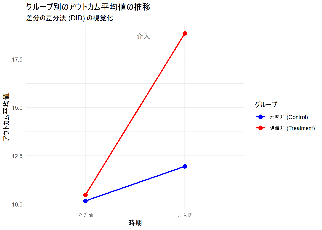
各グループ・時期の平均値および DID推定値 を求めます。
result_did <- function() {
  mean_control_pre <- summary_df %>%
    filter(treatment_group == 0, time == 0) %>%
    pull(mean_outcome)
  mean_control_post <- summary_df %>%
    filter(treatment_group == 0, time == 1) %>%
    pull(mean_outcome)
  diff_control <- mean_control_post - mean_control_pre
  mean_treatment_pre <- summary_df %>%
    filter(treatment_group == 1, time == 0) %>%
    pull(mean_outcome)
  mean_treatment_post <- summary_df %>%
    filter(treatment_group == 1, time == 1) %>%
    pull(mean_outcome)
  diff_pre <- mean_treatment_pre - mean_control_pre
  diff_treatment <- mean_treatment_post - mean_treatment_pre
  did_estimate <- diff_treatment - diff_control
  list("対照群の介入前平均" = mean_control_pre, "対照群の介入後平均" = mean_control_post, "対照群の変化量" = diff_control, "処置群の介入前平均" = mean_treatment_pre, "処置群の介入後平均" = mean_treatment_post, "処置群の変化量" = diff_treatment, "介入前における、処置群と対照群のアウトカム平均の差" = diff_pre, "DID推定値 (処置群の変化量 - 対照群の変化量)" = did_estimate, "データ生成時の処置効果(再掲)" = treatment_effect)
}
result_did()
$対照群の介入前平均
[1] 10.16837
$対照群の介入後平均
[1] 11.95537
$対照群の変化量
[1] 1.786998
$処置群の介入前平均
[1] 10.48964
$処置群の介入後平均
[1] 18.82903
$処置群の変化量
[1] 8.339387
$`介入前における、処置群と対照群のアウトカム平均の差`
[1] 0.3212768
$`DID推定値 (処置群の変化量 - 対照群の変化量)`
[1] 6.552389
$`データ生成時の処置効果(再掲)`
[1] 6.5回帰分析により DID推定値 を求めることもできます。
回帰分析による DID では、相互作用項が DID推定値 に対応します。
\[\mathrm{outcom}=\beta_0+\beta_1\cdot\mathrm{treatment\_group}+\beta_2\cdot\mathrm{time} + \beta_3(\mathrm{treatment\_group} \cdot \mathrm{time}) + \epsilon\]
# 回帰モデルの実行
# time も treatment_group も 0/1 のダミー変数として投入
# 相互作用項 treatment_group:time の係数が DID 推定値となる
did_model <- lm(outcome ~ treatment_group + time + treatment_group:time, data = df)
# did_model <- lm(outcome ~ treatment_group * time, data = df)
summary(did_model)
did_estimate_regression <- coef(did_model)["treatment_group:time"]
list("回帰モデルから得られたDID推定値 (treatment_group:time の係数)" = did_estimate_regression)
Call:
lm(formula = outcome ~ treatment_group + time + treatment_group:time,
    data = df)

Residuals:
    Min      1Q  Median      3Q     Max
-8.7996 -2.0729  0.0088  1.8603  8.0384

Coefficients:
                     Estimate Std. Error t value Pr(>|t|)
(Intercept)           10.1684     0.2810  36.189  < 2e-16 ***
treatment_group        0.3213     0.3974   0.809    0.419
time                   1.7870     0.3974   4.497 9.06e-06 ***
treatment_group:time   6.5524     0.5620  11.660  < 2e-16 ***
---
Signif. codes:  0 '***' 0.001 '**' 0.01 '*' 0.05 '.' 0.1 ' ' 1

Residual standard error: 2.81 on 396 degrees of freedom
Multiple R-squared:  0.612, Adjusted R-squared:  0.609
F-statistic: 208.2 on 3 and 396 DF,  p-value: < 2.2e-16

$`回帰モデルから得られたDID推定値 (treatment_group:time の係数)`
treatment_group:time
            6.552389
ここで、
- (Intercept): β0。対照群(treatment_group=0)の介入前(time=0)のアウトカム平均の推定値。
- treatment_group: β1。介入前(time=0)における、処置群と対照群のアウトカム平均の差 (処置群 - 対照群)。
- time: β2。対照群における、介入前から介入後へのアウトカム平均の変化量(時間トレンド効果の推定値)。
- treatment_group:time: β3。DID推定値。対照群の時間変化に比べて、処置群で「追加的に」生じた介入後の変化量。これが介入効果の推定値となる。
最後に treatment_effect = 0 とした場合を確認します(並行トレンド仮説の確認)。
set.seed(seed)

treatment_effect <- 0

baseline_outcome <- rnorm(n_per_group * 2, mean = baseline_mean, sd = sd_noise)

df <- expand.grid(
  id = 1:(n_per_group * 2),
  time = 0:(time_points - 1)
) %>%
  as_tibble() %>%
  arrange(id, time) %>%
  mutate(
    treatment_group = ifelse(id > n_per_group, 1, 0)
  ) %>%
  mutate(
    baseline_y = baseline_outcome[id],
    outcome = baseline_y +
      time * time_trend_effect +
      treatment_group * time * treatment_effect +
      rnorm(n(), mean = 0, sd = sd_noise)
  ) %>%
  select(-baseline_y)

summary_df <- df %>%
  group_by(treatment_group, time) %>%
  summarise(mean_outcome = mean(outcome), .groups = "drop")

plot_trends()
result_did()
$対照群の介入前平均
[1] 10.16837
$対照群の介入後平均
[1] 11.95537
$対照群の変化量
[1] 1.786998
$処置群の介入前平均
[1] 10.48964
$処置群の介入後平均
[1] 12.32903
$処置群の変化量
[1] 1.839387
$`介入前における、処置群と対照群のアウトカム平均の差`
[1] 0.3212768
$`DID推定値 (処置群の変化量 - 対照群の変化量)`
[1] 0.05238889
$`データ生成時の処置効果(再掲)`
[1] 0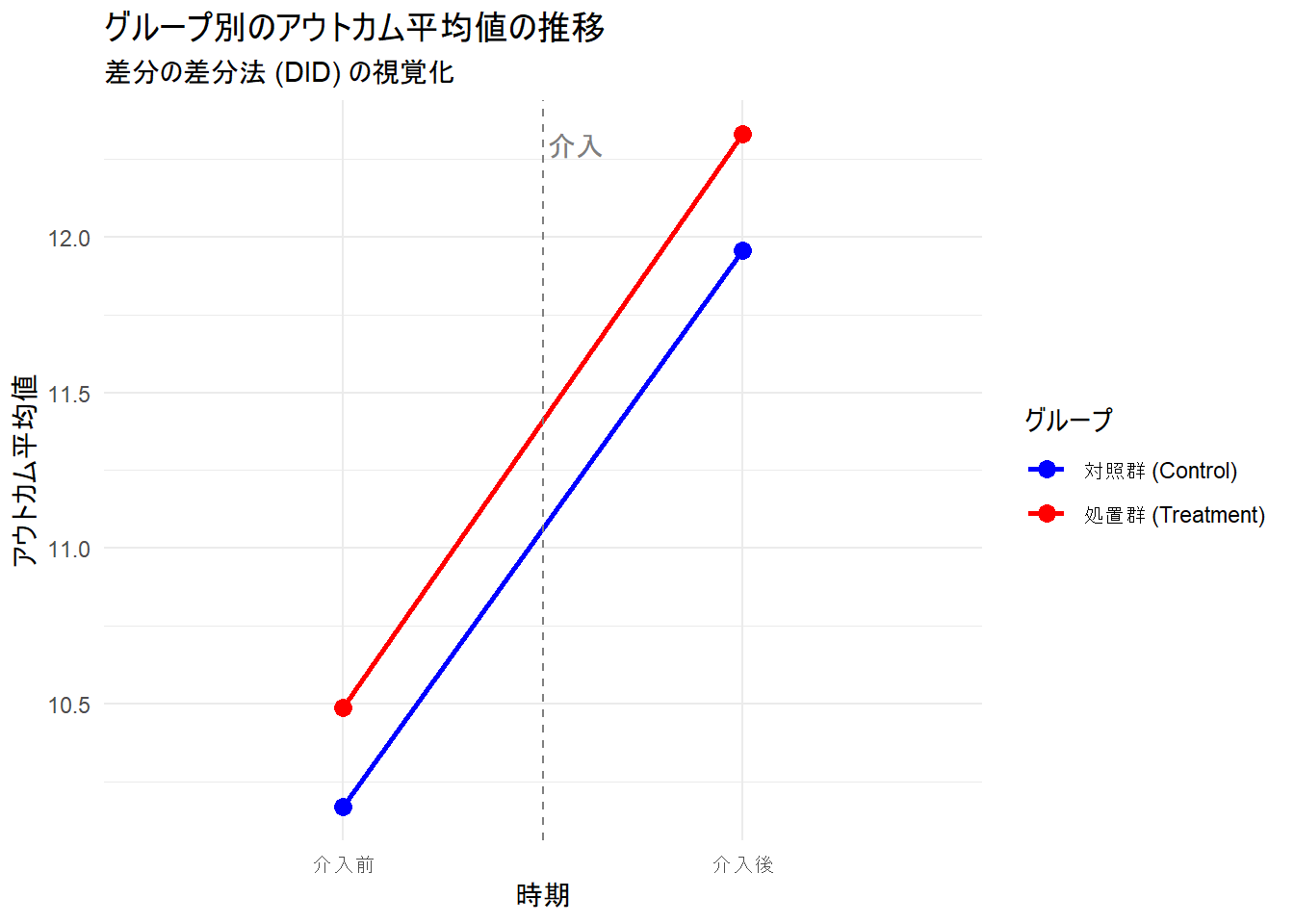
以上です。