
Rで Permutation test を試みます。
始めに平均値と分散の異なるAとBの2つのサンプルを作成します。
なお、それぞれのサンプルサイズは30未満(少数サンプル)とします。
seed <- 20250412
set.seed(seed = seed)

n_a <- 10
n_b <- 20

# 平均・分散が異なるガンマ分布から生成
# ガンマ分布の期待値 = 形状パラメータ × 尺度パラメータ
# ガンマ分布の分散 = 形状パラメータ × 尺度パラメータ^2
sample_a <- rgamma(n = n_a, shape = 2, rate = 0.1)
sample_b <- rgamma(n = n_b, shape = 4, rate = 0.1)

list(サンプルAの基本統計量 = summary(sample_a), サンプルAの標準偏差 = sd(sample_a), サンプルBの基本統計量 = summary(sample_b), サンプルBの標準偏差 = sd(sample_b))
$サンプルAの基本統計量
Min. 1st Qu. Median Mean 3rd Qu. Max.
6.19 11.46 18.35 19.73 23.24 47.39
$サンプルAの標準偏差
[1] 11.95069
$サンプルBの基本統計量
Min. 1st Qu. Median Mean 3rd Qu. Max.
14.89 23.34 34.50 36.72 52.33 66.73
$サンプルBの標準偏差
[1] 15.58654検定する統計量「サンプルAとサンプルBの平均値の差」を確認します
(obs_mean_diff <- mean(sample_a) - mean(sample_b))[1] -16.99448続いて Permutation test の関数を作成します。
permutation_test_mean_diff <- function(x, y, n_permutations) {
  n_x <- length(x)
  n_y <- length(y)
  combined_data <- c(x, y)
  n_total <- n_x + n_y
  observed_diff <- mean(x) - mean(y)
  perm_diffs <- numeric(n_permutations)

  for (i in 1:n_permutations) {
    # データをランダムに並び替え(インデックスをシャッフル)
    shuffled_indices <- sample(1:n_total)
    # 新しいグループA'とB'を作成
    perm_x <- combined_data[shuffled_indices[1:n_x]]
    perm_y <- combined_data[shuffled_indices[(n_x + 1):n_total]]

    # 順列データの平均値の差を計算
    perm_diffs[i] <- mean(perm_x) - mean(perm_y)
  }

  # p値の計算 (両側検定)
  extreme_count <- sum(abs(perm_diffs) >= abs(observed_diff))
  # sample_a と sample_b 自体もカウントする場合は
  # p_value <- (extreme_count + 1) / (n_permutations + 1)
  p_value <- extreme_count / n_permutations

  list(
    observed_difference = observed_diff,
    p_value = p_value,
    n_permutations = n_permutations,
    permuted_differences = perm_diffs
  )
}
Permutation test の結果を確認します。
set.seed(seed = seed)
result <- permutation_test_mean_diff(x = sample_a, y = sample_b, n_permutations = 10000)
result$p_value
[1] 0.0053「サンプルAとサンプルBの平均値は同一」との帰無仮説は有意水準5%で棄却されます。
シミュレーションの結果を可視化します。
library(dplyr)
library(ggplot2)
ggplot(mapping = aes(x = result$permuted_differences)) +
  geom_histogram(color = "white") +
  geom_vline(xintercept = result$observed_difference, color = "red")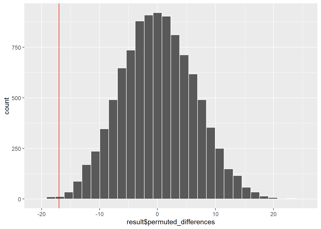
Rの関数 perm {perm} を利用した Permutation test です。
library(perm)
control <- permControl(nmc = 10000)
permTS(x = sample_a, y = sample_b, alternative = "two.sided", exact = FALSE, control = control)
    Permutation Test using Asymptotic Approximation

data:  sample_a and sample_b
Z = -2.671, p-value = 0.007563
alternative hypothesis: true mean sample_a - mean sample_b is not equal to 0
sample estimates:
mean sample_a - mean sample_b
-16.99448 「サンプルAとサンプルBの平均値は同一」との帰無仮説は有意水準5%で棄却されます。
なお、シミュレーション(サンプリング)が異なりますのでp値は一致しません。
もう一つサンプルを作成します。
# 平均・分散が同一の一様分布から生成
# 連続一様分布の期待値 = (min + max)/2
# 連続一様分布の分散 = (max - min)^2/12
set.seed(seed = seed)
sample_a <- runif(n = n_a, min = 0, max = 20)
sample_b <- runif(n = n_b, min = 0, max = 20)

list(サンプルAの基本統計量 = summary(sample_a), サンプルAの標準偏差 = sd(sample_a), サンプルBの基本統計量 = summary(sample_b), サンプルBの標準偏差 = sd(sample_b))
result <- permutation_test_mean_diff(x = sample_a, y = sample_b, n_permutations = 10000)
result$p_value
$サンプルAの基本統計量
Min. 1st Qu. Median Mean 3rd Qu. Max.
2.251 4.388 6.918 9.613 14.626 19.431
$サンプルAの標準偏差
[1] 6.386803
$サンプルBの基本統計量
Min. 1st Qu. Median Mean 3rd Qu. Max.
0.2668 3.9278 8.5445 8.3433 11.5284 19.9477
$サンプルBの標準偏差
[1] 5.04955
[1] 0.5539「サンプルAとサンプルBの平均値は同一」との帰無仮説は有意水準5%で棄却されません。
可視化します。
ggplot(mapping = aes(x = result$permuted_differences)) +
  geom_histogram(color = "white") +
  geom_vline(xintercept = result$observed_difference, color = "red")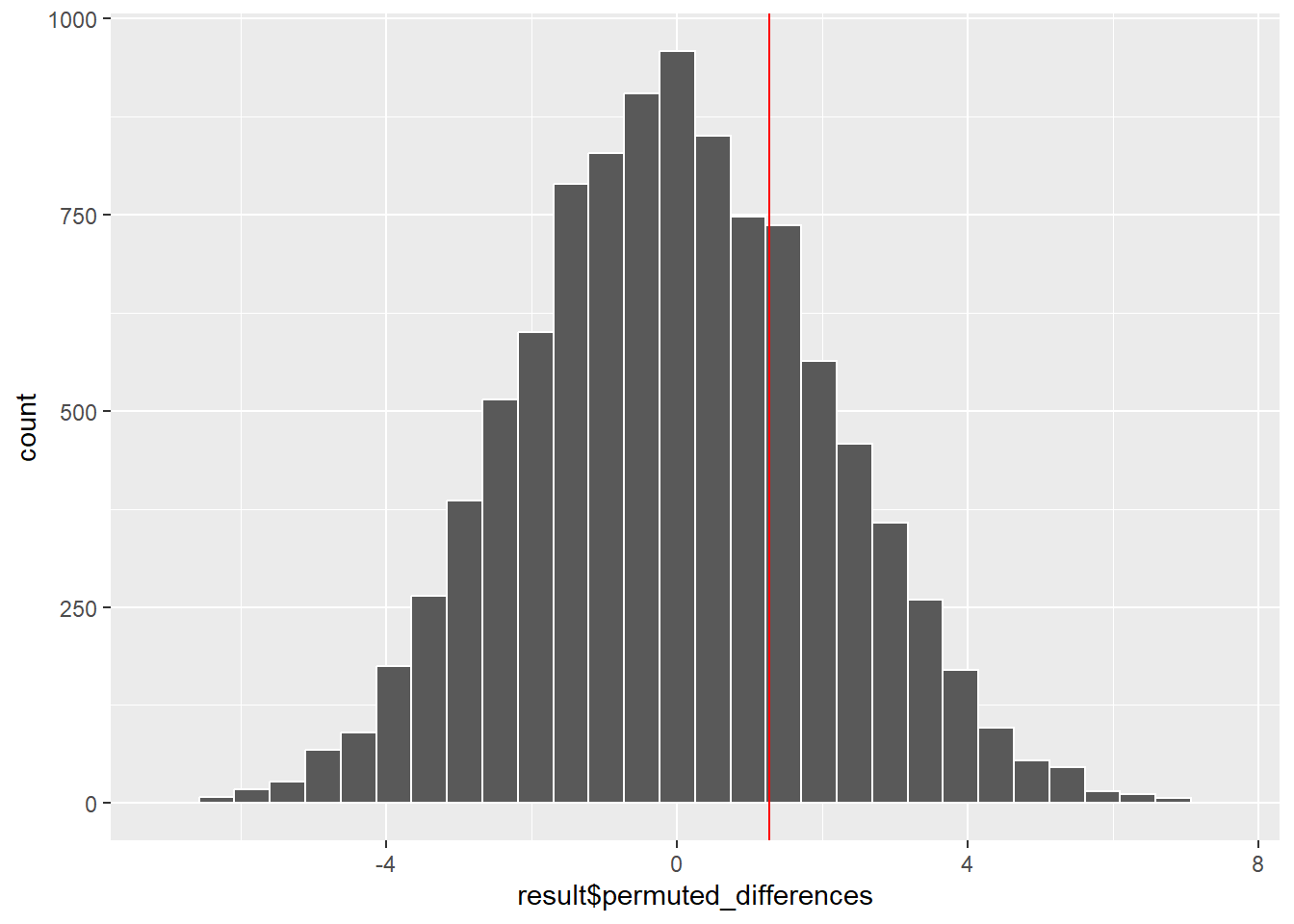
perm {perm} の結果を確認します。
control <- permControl(nmc = 10000)
permTS(x = sample_a, y = sample_b, alternative = "two.sided", exact = FALSE, control = control)
    Permutation Test using Asymptotic Approximation

data:  sample_a and sample_b
Z = 0.6014, p-value = 0.5476
alternative hypothesis: true mean sample_a - mean sample_b is not equal to 0
sample estimates:
mean sample_a - mean sample_b
                     1.270128
同じく棄却されません。
以上です。