AICを利用してloess{stats}の最適spanを選択

こちらの続きです。

RでLOESS-locally estimated scatterplot smoothing-

loess {stats} を利用して平滑化する際の最適スパンを AIC(Akaike Information Criterion) を利用して選択します。

参照引用しました資料は以下の通りです。

Clifford M. Hurvich, Jeffrey S. Simonoff, Chih-Ling Tsai, Smoothing Parameter Selection in Nonparametric Regression Using an Improved Akaike Information Criterion, Journal of the Royal Statistical Society Series B: Statistical Methodology, Volume 60, Issue 2, July 1998, Pages 271–293
https://support.sas.com/documentation/onlinedoc/stat/131/loess.pdf
https://github.com/SurajGupta/r-source/blob/master/src/library/stats/src/loessc.c
https://github.com/SurajGupta/r-source/blob/master/src/library/stats/R/loess.R
https://github.com/bluegreen-labs/phenocamr/blob/master/R/optimal_span.r

始めにサンプルデータを作成します。なお、LOESS回帰曲線 の span はデフォルトの 0.75 とします。

library(dplyr)
library(ggplot2)
set.seed(20240816)
x <- seq(0, 5 * pi, 0.01)
y <- (sin(x = x) + rnorm(n = length(x), sd = 0.5))
g <- ggplot(mapping = aes(x = x, y = y)) +
  geom_point(size = 1)
g + geom_smooth(method = loess, method.args = list(degree = 2, span = 0.75, family = "gaussian", method = "loess"), se = F, linewidth = 1.2)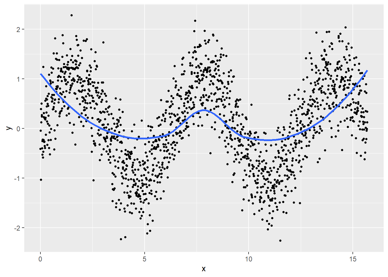

上記 資料2 の \(\mathrm{AIC}_{c1}\) を最適スパン選択に利用します。

\[\mathrm{AIC}_{C1}=n\,\mathrm{log}\left(\hat{\sigma}^2\right)+n\dfrac{\delta_1/\delta_2\left(n+\nu_1\right)}{\delta_1/\delta_2-2}\] ここで、

\[\begin{eqnarray} n&:&\mathrm{Number\, of\, observations}\,(サンプルサイズ)\\ \mathbf{L}&:&\mathrm{Smoothing\, Matrix}\,(平滑化行列),\quad\hat{\mathbf{y}}=\mathbf{Ly} \end{eqnarray}\] を表し、\(\delta_1,\delta_2,\nu_1\) はそれぞれ \[\begin{eqnarray} \delta_1&\equiv&\mathrm{Trace}\left(\left(\mathbf{I}-\mathbf{L}\right)^\mathsf{T}\left(\mathbf{I}-\mathbf{L}\right)\right)\\ \delta_2&\equiv&\mathrm{Trace}\left(\left(\mathbf{I}-\mathbf{L}\right)^\mathsf{T}\left(\mathbf{I}-\mathbf{L}\right)\right)^2\\ \nu&\equiv&\mathrm{Trace}\left(\mathbf{L}^\mathsf{T}\mathbf{L}\right),\quad \mathrm{Equivalent\, Number\, of\, Parameters}\,(等価パラメータ数) \end{eqnarray}\] として求められます。

span のレンジは 0.01 から 0.01 刻みで最大 1 とします。

AICc1 <- vector()
cnt <- 1
span.vec <- seq(0.01, 1, by = 0.01)
for (span in span.vec) {
  result.loess <- loess(y ~ x, span = span)
  n <- result.loess$n
  sigma2 <- sum(result.loess$residuals^2) / (n - 1)
  delta1 <- result.loess$one.delta
  delta2 <- result.loess$two.delta
  equivalent.number.of.parameters <- result.loess$enp
  AICc1[cnt] <- n * log(sigma2) + n * delta1 / delta2 * (n + equivalent.number.of.parameters) / (delta1^2 / delta2 - 2)
  cnt <- cnt + 1
}
ggplot(mapping = aes(x = span.vec, y = AICc1)) +
  geom_bar(stat = "identity")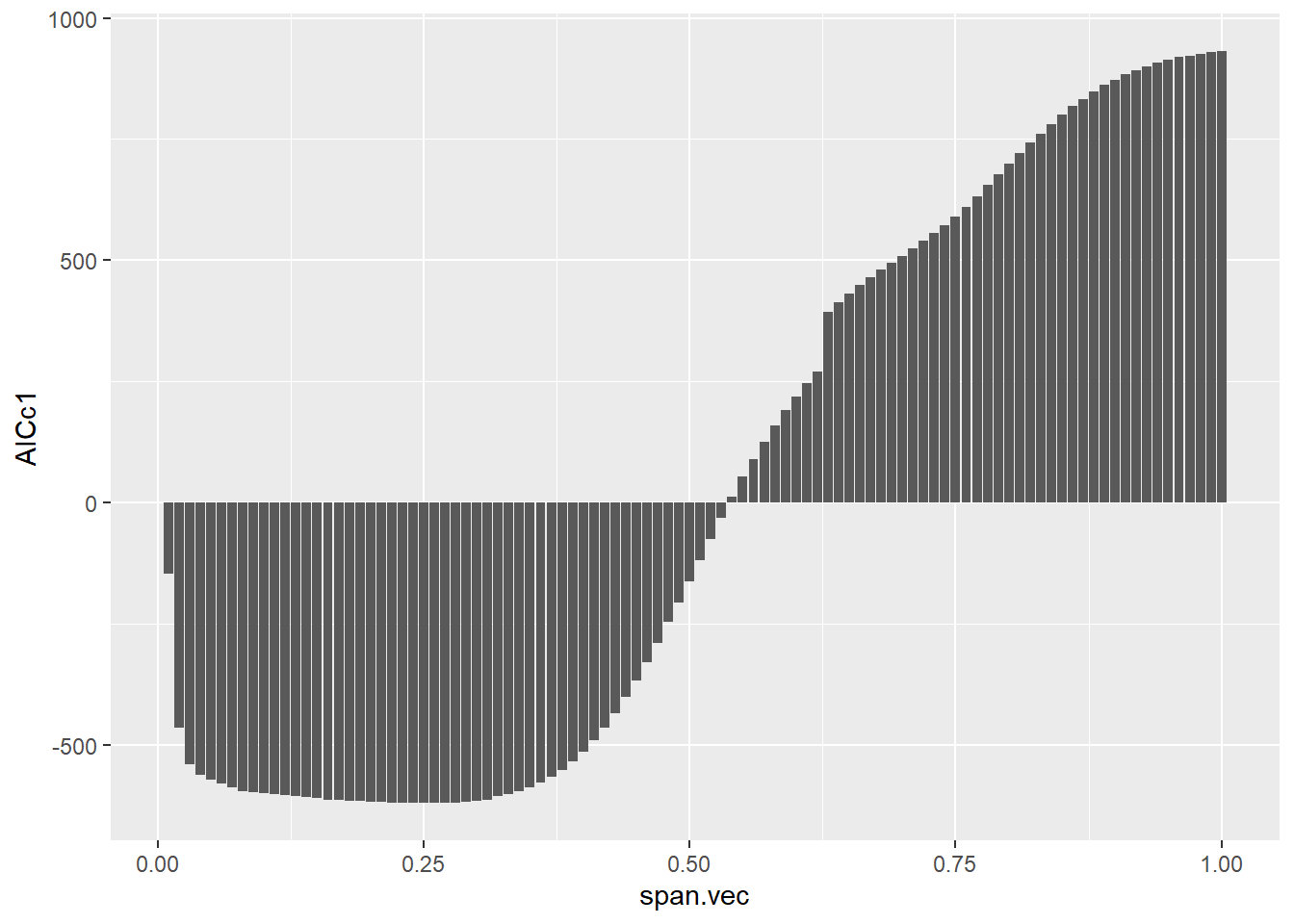

最小の AICc1 を確認します。

optimal.span <- AICc1 %>%
  which.min() %>%
  span.vec[.]
optimal.span

[1] 0.26

求めた最適スパン(AICc1 が最小となったスパン)を用いて LOESS回帰曲線 を描きます。

g + geom_smooth(method = loess, method.args = list(degree = 2, span = optimal.span, family = "gaussian", method = "loess"), se = F, linewidth = 1.2)

`geom_smooth()` using formula = 'y ~ x'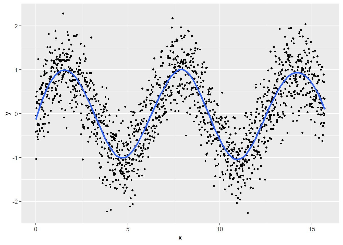

以上です。