自己回帰モデルのパラメータの変化による単位根および自己相関検定の結果の相違
更新日時:2019-04-29 19:17:31
Content
set.seed(seed = '20181231')
library(tseries)
resultdf <- data.frame()
cnt <- 1
for(a in seq(-1.5,1.5,0.25)){
  pvalue <- pvalue_diff <- vector()
  for(iii in seq(10)){
    y <- vector();y[1] <- 0
    for(t in 2:50){
      y[t] <- a*y[t-1] + rnorm(n = 1)
    }
    pvalue[iii] <- round(adf.test(x = y)$p.value,2)
    pvalue_diff[iii] <- round(adf.test(x = diff(y))$p.value,2)
  }
  resultdf[cnt,1] <- a
  resultdf[cnt,2] <- paste0(sort(unique(pvalue)),collapse = ',')
  resultdf[cnt,3] <- paste0(sort(unique(pvalue_diff)),collapse = ',')
  resultdf[cnt,4] <- Box.test(y,lag = 1,type = "Ljung-Box")$p.value
  resultdf[cnt,5] <- Box.test(diff(y),lag = 1,type = "Ljung-Box")$p.value
  cnt <- cnt + 1
}
colnames(resultdf) <- c('a','p value of ADF test:Level data','p value of ADF test:1st difference','p value of Ljung-Box test:Level data,lag=1','p value of Ljung-Box test:1st difference data,lag=1')| a | p value of ADF test:Level data | p value of ADF test:1st difference | p value of Ljung-Box test:Level data,lag=1 | p value of Ljung-Box test:1st difference data,lag=1 |
|---|---|---|---|---|
| -1.5 | 0.01,0.12 | 0.01 | 0.0000012 | 0.0000015 |
| -1.25 | 0.01,0.02,0.03,0.06,0.41 | 0.01 | 0 | 0 |
| -1 | 0.01,0.05,0.06,0.09,0.24,0.36 | 0.01 | 0 | 0 |
| -0.75 | 0.01,0.02,0.04,0.05,0.06 | 0.01 | 0 | 0 |
| -0.5 | 0.01,0.02,0.09 | 0.01 | 0.0002503 | 0 |
| -0.25 | 0.01,0.02,0.03,0.19,0.24,0.25,0.3 | 0.01 | 0.0105692 | 0.0000002 |
| 0 | 0.01,0.03,0.08,0.1,0.21,0.27 | 0.01 | 0.0193697 | 0.0000108 |
| 0.25 | 0.01,0.03,0.04,0.05,0.09,0.1,0.18,0.3 | 0.01 | 0.0251779 | 0.2510908 |
| 0.5 | 0.01,0.03,0.06,0.1,0.16,0.17,0.28,0.29,0.37 | 0.01,0.02 | 0.0016714 | 0.0323443 |
| 0.75 | 0.04,0.06,0.08,0.14,0.17,0.2,0.34,0.35,0.4 | 0.01,0.02,0.27 | 0.0000032 | 0.812635 |
| 1 | 0.04,0.06,0.29,0.46,0.59,0.76,0.81,0.87,0.91,0.99 | 0.01,0.02,0.04,0.1,0.17,0.36 | 0 | 0.762884 |
| 1.25 | 0.99 | 0.99 | 0 | 0 |
| 1.5 | 0.99 | 0.99 | 0.0000013 | 0.0000016 |
\(\,\,a=1\,\,\)でもp値が0.04、\(\,\,a=0\,\,\)でもp値が0.27と出る場合があります。続いて改めてパラメータ\(\,\,a\,\,\)の変化による時系列チャートの形状、そしてそれぞれの単位根検定と自己相関検定のp値の例を確認してみましょう。
fun_plot <- function(x,maintitle,h,xlab,ylim){
  plot(x = x,type = 'o',panel.first = grid(nx = NULL,ny = NULL,lty = 2,equilogs = T),xlab = xlab,ylim=ylim)
  title(main = maintitle,line = 1,cex.main = 1)
  abline(h = h,col = 'red')
}
for(a in seq(-1.5,1.5,0.25)){
  y <- vector();y[1] <- 0
  for(t in 2:50){
    y[t] <- a*y[t-1] + rnorm(n = 1)
  }
  cat(paste0('<div align="center"><b>a = ',a,'</b></div>'))
  par(mfrow=c(2,3),oma=c(0,0,4,0))
  for(iii in 1:6){
    if(iii%%3==1){
      h <- 0;xlab <- 't'
      if(iii==1){x <- y;maintitle0 <- 'Level'}
      if(iii==4){x <- diff(y);maintitle0 <- '1st difference'}
      maintitle <- paste0('Time Series(',maintitle0,')\np value of ADF test=',round(adf.test(x = x)$p.value,2))
      ylim <- range(x)
    }
    if(iii%%3==2){
      pacf(x = x, ci = 0.95,main=maintitle0,lag.max = 10)
    }
    if(iii%%3==0){
      h <- 0.05;pvalue <- vector();xlab <- 'lag';ylim <- c(0,1)
      maintitle <- paste0('p value of Ljung-Box test\n',maintitle0)
      for(lag in 1:10){
        pvalue[lag] <- Box.test(x = x,lag = lag,type = "Ljung-Box")$p.value
      }
      x <- pvalue
    }
    if(iii%%3!=2){fun_plot(x = x,maintitle = maintitle,h = h,xlab = xlab,ylim = ylim)}
    mtext(text = paste0('a = ',a), side = 3, line = 0, outer = T,cex=1.1)
  }
  cat('<hr class="bar1">')
}
a = -1.5

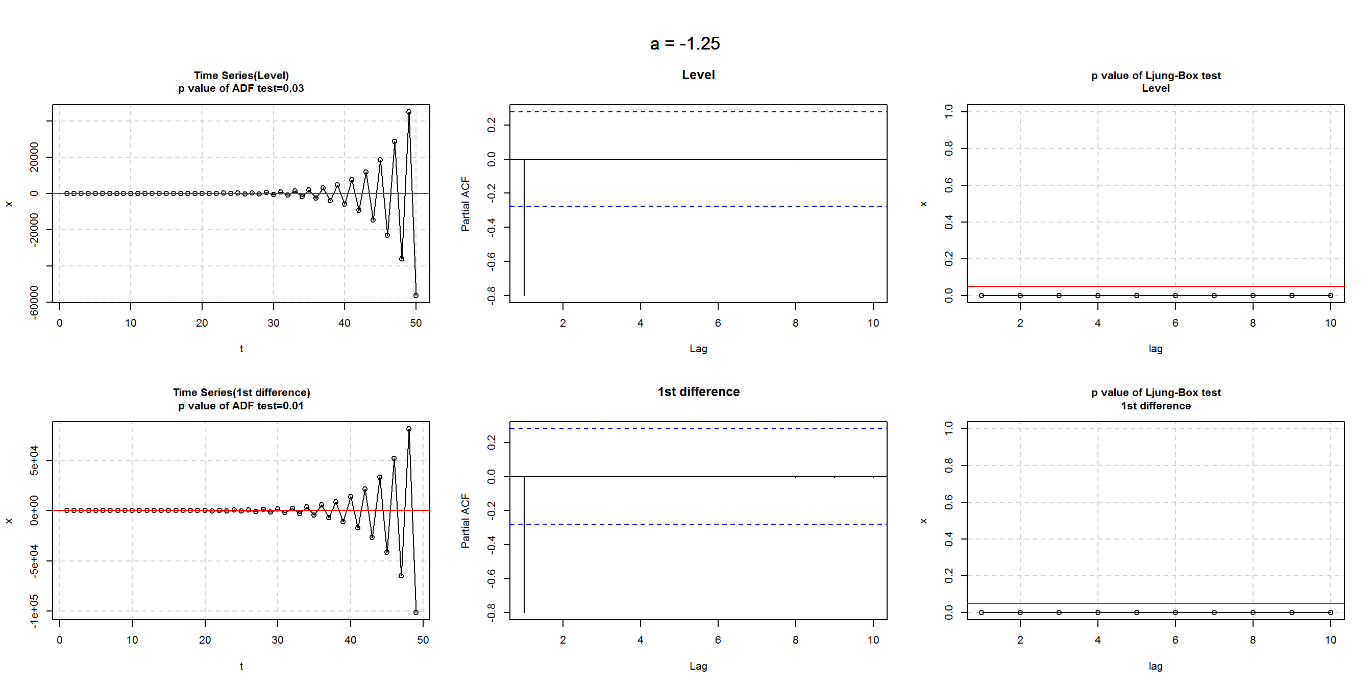
a = -1.25
a = -1

a = -0.75

a = -0.5

a = -0.25

a = 0

a = 0.25

a = 0.5

a = 0.75

a = 1

a = 1.25

a = 1.5

時系列データ分析に際して問題となるのが単位根。そこで\(\,\,\, y_{t}= a \times y_{t-1}+\varepsilon_{t}\) のAR(1)過程を例としてパラメータ\(\,\,a\,\,\)の変化による単位根検定、自己相関検定の結果および時系列チャート形状の相違を確認してみましょう。なおADF testの\(\,\,H_{0}\,\,\)は「非定常」、Box testの\(\,\,H_{0}\,\,\)は「自己相関なし」です。